Munich Personal RePEc Archive
Semiparametric penalty function method
in partially linear model selection
Dong, Chaohua and Gao, Jiti and Tong, Howell
The University of Adelaide, The University of Adelaide, London
School of Economics
February 2006
Online at
https://mpra.ub.uni-muenchen.de/11975/
Munich Personal RePEc Archive
Semiparametric penalty function method
in partially linear model selection
Dong, Chaohua, Gao, Jiti and Tong, Howell
The University of Adelaide, The University of Adelaide,
London School of Economics
February 2006
Online at
http://mpra.ub.uni-muenchen.de/11975/
Semiparametric Penalty Function Method in Partially
Linear Model Selection
By Chaohua Dong, Jiti Gao1 and Howell Tong
Shanxi University of Economics and Finance; The University of Western Australia;
The London School of Economics
Abstract: Model selection in nonparametric and semiparametric regression is of both theoretical and practical interest. Gao and Tong (2004) proposed a semiparametric leave– more–out cross–validation selection procedure for the choice of both the parametric and nonparametric regressors in a nonlinear time series regression model. As recognized by the authors, the implementation of the proposed procedure requires the availability of relatively large sample sizes. In order to address the model selection problem with small or medium sample sizes, we propose a new model selection procedure for practical use. By extending the so–called penalty function method proposed in Zheng and Loh (1995, 1997) through the incorporation of features of the leave-one-out cross-validation approach, we develop a semiparametric consistent selection procedure suitable for the choice of optimum subsets in a partially linear model. The newly proposed method is implemented using the full set of the data, and simulations show that it works well for both small and medium sample sizes.
1. Introduction
The problem of model selection in linear, nonlinear and partially linear regression models has attracted much attention in recent years. Many selection methods have been developed since the pioneering notions of Akaike’s information criterion (AIC) (Akaike (1974); Shibata (1981)) and Mallows’Cp (Mallows (1973)). Recent developments that address the nonlinear and partially linear cases include leave–one–out cross-validation (CV1) (e.g. Cheng and Tong (1992); Vieu (1994); Yao and Tong (1994)), and leave–more–out cross–validation (e.g. Shao (1993); Zhang (1993); Gao and Tong (2004)). Usually a model selection method is to select the true subset of covariates for either a given dependent variable or a collection of covariates. The most commonly adopted strategy consists of two components: the residual
sum of squares (RSS) (as a measure of the goodness of fit) and some function of the number of covariates in the candidate model (as a measure of the penalty for model complexity). By minimizing the sum of these two components, sometimes called the final prediction error, we aim to identify the true model.
Asymptotic consistency is obtained for the fully nonparametric CV1 model selection (e.g. Cheng and Tong (1992)), but in a parametric setting the leave–one–out cross–validation tends to lead to an inconsistent selection and is considered to be too conservative in the sense that it tends to select an unnecessarily large model. In order to restore consistency, Shao (1993) proposed the so–called leave–more–out cross–validation, denoted by CV(Tv) with Tv
T →1, where T is the number of observations and Tv the number of observations removed for cross-validation. Recently, Gao and Tong (2004) extended this method to semiparametric time series modelling. As observed in the simulations in both Shao (1993) and Gao and Tong (2004), the number of observations, Tc, used to fit the model is quite small (with T = 40 and Tc = 15 in Shao (1993), and T = 288 and Tc = 69 in Gao and Tong (2004)), while the number of observations, Tv, used to validate the proposed method is relatively large (with
Tv = 25 and Tv = 219, respectively). This may impede the implementation of the above methodology in practice because the theory requires Tc → ∞. To ensure that more data are used to construct the model, Zheng and Loh (1995, 1997) proposed using a parametric penalty function method. Such observations have motivated us to consider combining the penalty function method proposed in Zheng and Loh (1995, 1997) with the CV1 method for semiparametric modelling. The use of semiparametric models has become increasingly popular in statistical modelling, mainly because these models are quite effective in dealing with the problem of curse of dimensionality, that often arises from using fully nonparametric models.
Specifically, we consider a partial linear model of the form
Yt =Utτβ+φ(Xt) +et, t= 1,· · ·, T, (1.1)
where Ut = (Ut1, . . . , Utp)τ and Xt = (Xt1, . . . , Xtq)τ are vectors of either independent or dependent observations (Ut and Xt may be two different time series), β = (β1, . . . , βp)τ is a vector of unknown parameters,φ(·) is an unknown and possibly nonlinear function defined over Rq, and the error process {e
model selection criterion, by incorporating essential features of the CV1 selection method for the choice of both the parametric and the nonparametric regressors in model (1.1). Our contributions include proposing a new selection criterion, developing the associated theory, and demonstrating the key feature of easy implementation of the proposed semiparametric penalty function method through using simulated examples. The organization of this paper is as follows. Section 2 proposes the penalty–function–based selection criterion and develops its asymptotic theory. Two simulated examples are given in Section 3. Assumptions and proofs are given in the appendix.
2. Semiparametric penalty function method
First we introduce some notation. Let Ap = {1,· · ·, p}, Dq = {1,· · ·, q}, A denote all nonempty subsets of Ap, and D denote all nonempty subsets of Dq. For any subset
A ∈ A, UtA is defined as a column vector consisting of {Uti, i ∈ A}, and βA is the column vector consisting of {βi, i∈A}. For any subsetD ∈ D, XtD is the column vector consisting of {Xti, i∈D}.We use dE =|E| to denote the cardinality of a set E. Let
A1 = {A :A ∈ A such that at least one nonzero component ofβ is not inβA}
A2 = {A :A ∈ A such thatβA contains all nonzero component of β}
D1 = {D:D∈ D such that E[Yt|XtD] =E[Yt|Xt]}
D2 = {D:D∈ D such that E[Utτβ|XtD] =E[Utτβ|Xt]}
B1 = {(A, D) :A∈ A2 and D∈ D1∩ D2}.
Obviously, the subsetsA∈ A1 andD∈ Dc1 =D−D1correspond to incorrect models. The
correct models correspond to (A0, D0) ∈ B1 such that both A0 and D0 are of the smallest
dimension. To ensure the existence and uniqueness of such a pair (A0, D0), we need the
same conditions as required in Gao and Tong (2004). For the sake of being self–contained, we recite them here.
Assumption 2.1. (i) ∆A,D =E{UtA−E[UtA|XtD]}{UtA−E[UtA|XtD]}τ is a positive definite matrix of order dA×dA for each given pair of A∈ A and D∈ D.
(ii) Let B0 = {(A0, D0) ∈ B1,such that|A0|+|D0| = min(A,D)∈B1[|A|+|D|]}. The pair
Assumption 2.2. There is a unique pair (β∗, φ∗) such that the true and compact version of model (1.1) is
Yt=UtAτ ∗β∗+φ∗(XtD∗) +et, (2.1)
whereet =Yt−E[Yt|Ut, Xt].
Assumption 2.3. Define θj(Xtj) = E[φ∗(XtD∗)|Xtj] for j ∈ Dq − D∗. There exists an
absolute constant M0 such that
min
j∈Dq−D∗minα,β E[θj(Xtj)
−α−βXtj]2 ≥M0. (2.2)
Assumption 2.1 is a standard condition in this kind of problem. Assumption 2.2 is to ensure the existence and uniqueness of the true model. Assumption 2.3 is imposed to ensure that model (2.1) is identifiable and to exclude the case in whichφ∗ itself is a linear function inXtj forj ∈Dq−D∗. More details are available in Gao and Tong (2004).
For any given pair A∈ A and D∈ D, we consider a partial linear model of the form
Yt=UtAτ βA+φD(XtD) +et(A, D), (2.3)
where et(A, D) = Yt − E[Yt|UtA, XtD], βA is as defined before, and φD(·) is an unknown function on R|D|.
To use CV1, we introduce some notation to smooth and linearize the semiparametric model (2.3):
ˆ
φ1t(D) = T
X
s=1,s6=t
WD(−t)(t, s)Ys, φˆ2t(A, D) = T
X
s=1,s6=t
WD(−t)(t, s)UsA,
Zt(D) =Yt−φˆ1t(D), Z(D) = (Z1(D),· · ·, ZT(D))τ,
Vt(A, D) =UtA−φˆ2t(A, D), V(A, D) = (V1(A, D),· · ·, VT(A, D))τ,
φ1(Xt) = E[Yt|Xt], φ2(Xt) = E[Ut|Xt],
Vt=Ut−φ2(Xt), V = (V1,· · ·, VT)τ, (2.4)
where
WD(−t)(t, s) =
KD((XtD−XsD)/h)
PT
l=1,l6=tKD((XtD−XlD)/h)
in which T is the number of observations, KD is a multivariate kernel function defined on
R|D|, and h =h
D is a bandwidth parameter satisfying h∈ HT D = [hmin(T, D), hmax(T, D)],
where both 0 < hmin(T, D), hmax(T, D) ≤ 1 are suitable functions of (D, T) such that the
optimal order T−4+1|D| is included in H
T D. In the conventional cross–validation selection of an optimal bandwidth for the autoregressive case, the optimal bandwidth is proportional to
σ T−15 for example, where σ is the standard deviation of the data.
A technical advantage of using HT D over previous assumptions of this type, such as an interval of the form
c1 T−
7 6(4+|D|), c
2 T−
5 6(4+|D|)
with 0 < c1 < c2 < ∞, as proposed in Gao
and Yee (2000), is that the range ofh under consideration has been extended considerably. This provides more security and theoretical underpinning for consideration of h both large and small, as initially discussed in H¨ardle, Hall and Marron (1992). In addition, Lemma A.1(i) in the appendix shows that an optimal choice ofh depends mainly on the choice ofD
and T. This is why we do not involveh in the penalty function ΛT(A, D) to be introduced in Assumption 2.4 below.
We set up the linearized model
Zt(D) = Vt(A, D)βA+et(A, D), (2.5)
and give the least squares estimator ofβA as
ˆ
β(A, D) =V(A, D)τV(A, D)+V(A, D)τZ(D), (2.6)
where (·)+ is the Moore-Penrose inverse.
After fitting (2.5) to the data {(Yt, Ut, Xt) :t= 1,· · ·, T}, the residual sum of squares is
RSS(A, D;h) = T
X
t=1
h
Zt(D)−Vt(A, D)τβˆ(A, D)
i2
(2.7)
=Z(D)−V(A, D) ˆβ(A, D)τZ(D)−V(A, D) ˆβ(A, D)
=ετR(A, D)ε+ ˜Φ(D)τR(A, D) ˜Φ(D) + (V β)τR(A, D)(V β) + ∆T(A, D;h),
where ε= (e1,· · ·, eT)τ, P(A, D) =V(A, D)(V(A, D)τV(A, D))+V(A, D)τ, R(A, D) =IT −
P(A, D),Φ(˜ D) = ( ˜φ1(D),· · ·,φ˜T(D))τ,φ˜t(D) = φ1(Xt)−φˆ1t(D), IT is the identity matrix of orderT ×T, and the reminder term is
It may be shown from (2.7) that the following equations hold uniformly in h∈HT D,
RSS(A, D;h) =ετR(A, D)ε+ ˜Φ(D)τR(A, D) ˜Φ(D) + (V β)τR(A, D)(V β) +oP(RSS(A, D;h)),
MT(A, D;h) =E[RSS(A, D;h)] = (T − |A|)σ2+PT(A, D) +NT(A, D) +o(MT(A, D)), (2.9)
wherePT(A, D) =E[(V β)τR(A, D)(V β)] andNT(A, D) =E
h
˜
Φ(D)τR(A, D) ˜Φ(D)i. Then equa-tions in (2.9) reflect the errors incurred in model selection and estimation. The proof of (2.9) is relegated to Lemma A.3 in the appendix.
The penalty function ΛT(A, D) is now defined as
ΛT(A, D) :A × D → R,
and satisfies the following assumption.
Assumption 2.4. (i) Let ΛT(∅, D) = 0 forD =∅ or any givenD ∈ D. (ii) For any subsets A1, A2 ∈ A, D1, D2 ∈ D satisfying A2 ⊃A1, D2 ⊃D1,
lim T→∞inf
ΛT(A1, D1)
ΛT(A2, D2)
<1.
(iii) For any nonempty sets A and D,
lim
T→∞ΛT(A, D) =∞ and Tlim→∞
ΛT(A, D)
T = 0.
Remark 2.1. (i) It should be noted that ΛT(A, D) can be chosen quite generally. It is a function of sets in theory, but in practice we can define the penalty function as a function of |A| and |D| satisfying Assumption 2.4. Obviously, the definition of ΛT(A, D) generalizes the function hn(k) in Zheng and Loh (1997).
(ii) Assumption 2.4 regularizes the penalty function so as to avoid any problem of over-fitting or under-over-fitting.
We now extend the penalty function method from linear model selection to the partial linear model selection. Define
( ˆA,D,ˆ ˆh) = arg min A∈A,D∈D,h∈HT D
{RSS(A, D;h) + ΛT(A, D)σb2}, (2.10)
where σb2 = 1
T−pRSS(Ap, Dq;h) is the usual consistent estimate of Var[et] = σ
2. It may be
shown from equation (14) of Zheng and Loh (1997) that
b
uniformly inh∈HT D. The proof of (2.11) is similar to, but simpler, than that of (2.9) and is therefore omitted.
Remark 2.2. The method proposed in this paper generalizes those in Zheng and Loh (1995, 1997), Yao and Tong (1994), and Vieu (1994). For example, ifD∗ is already identified, then the problem becomes a model selection problem for linear models as discussed in Zheng and Loh (1995,1997). IfA is already identified as A∗, and we need only to select D for (A∗, D), then the model selection reduces to a purely nonparametric leave–one–out cross–validation selection problem. This is because, as shown in Section 2.1 of Gao and Tong (2002), the leading term T1RSS(A∗, D;h) is asymptotically equivalent to aCV1(D, h) function of (D, h) defined as
CV1(D, h) = 1
T
T
X
t=1
n
Yt−Utτβˆ(Ap, D)−φbt(XtD,βˆ(Ap, D))
o2
, (2.12)
whereφbt(XtD, β) = ˆφ1t(D)−φˆ2t(A, D)τβ and ˆβ(A, D) are given at (2.6). Thus, in the case whereA is already identified as A∗, we may choose (D, h) as follows:
( ˆD,ˆh) = arg min D∈D,h∈HT D
CV1(D, h).
We now state the main result of this paper; its proof is relegated to the Appendix.
Theorem 2.1. If the Assumptions 2.1–2.4 and A.1–A.5 of the Appendix hold, then
lim T→∞P
ˆ
A=A∗,Dˆ =D∗= 1 and hb
h∗ →P 1
as T → ∞, where h∗ =c∗T−4+|1D∗| and c
∗ is a positive constant.
3. Some simulation results
In this section we illustrate Theorem 2.1 using two simulated examples. Our simulation results support the asymptotic theory and the use of the semiparametric penalty function method for practical partial linear model selection.
Example 3.1. Consider a nonlinear time series model of the form
Yt = 0.47Ut−1−0.45Ut−2+
0.5Xt−1
1 +X2 t−1
+et,
where Ut = 0.55Ut−1 −0.12Ut−2 +δt and Xt = 0.3 sin(2πXt−1) +ǫt, in which δt, ǫt and
(−0.5,0.5) and N(0,1), respectively, U1, U2, X1, X2 are independent and identically
distrib-uted as uniform (−1,1), Us and Xt are mutually independent for all s, t ≥ 3, and the processes{(δt, ǫt, et) :t≥3} are independent of both (U1, U2) and (X1, X2).
For Example 3.1, the strict stationarity and mixing condition can be justified by using existing results (e.g. Masry and Tjøstheim (1995, 1997)). Thus, Assumption A.1 holds. For an application of Theorem 2.1, let
β = (β1, β2)τ = (0.47,−0.45)τ and φ(Xt−1) =
0.5Xt−1
1 +X2 t−1
.
In this example, we consider the case where Xt and Xt−1 are selected as candidate
non-parametric regressors and Ut−1 and Ut−2 as candidate parametric regressors. Then we use
(2.10) to check if (Ut−1, Ut−2, Xt−1) is the true set of semiparametric regressors. For this
case, there are 22−1 = 3 possible nonparametric regressors and 22−1 = 3 possible
para-metric regressors, respectively. Thus, there are 9 posisble candidates for the true model, since Ut and Xt are independent. Let D0 = {1}, D1 = {0}, D2 = {0,1},D = {Di : 0 ≤
i ≤ 2}, XtD0 =Xt−1, XtD1 = Xt, XtD2 = (Xt, Xt−1)
τ, A
0 = {1,2}, A1 = {1}, A2 = {2},A =
{Ai : i = 0,1,2}, UtA0 = (Ut−1, Ut−2)
τ, U
tA1 = Ut−1, and UtA2 = Ut−2. It follows that both
D∗ =D0 and A∗ =A0 are unique. Assumptions 2.1–2.3 therefore hold.
We use ΛT(A, D) = (|A|+|D|)·T0.5 as the penalty function. Thus, Assumption 2.4 holds automatically. In addition to this choice of ΛT(A, D), we also considered several other forms for ΛT(A, D). As the resulting simulated frequencies are very similar, we do not refer them here. Throughout Example 3.1, we use
h∈HT D0 =
c1 T−
7 6(4+|D0|), c
2 T−
5 6(4+|D0|)
=hT−307 , 2·T− 1 6
i
based on the method proposed in Gao and Yee (2000) withc1 = 1 andc2 = 2.
For the multivariate kernel function K(·) involved in WD(t, s), define k(u) = √12πe−
u2
2
and K(u1, . . . , uj) = Πji=1k(uj) forj = 1,2,3.
It follows that Assumptions A.1–A.4 are all satisfied. Now we prove that Assumption A.5 is also satisfied. Assumption A.5 (i) is checked in Gao and Tong (2004). The independence between Ut and Xt implies that E[UtAi|XtDj] = E[UtAi] for all i, j = 0,1,2. Thus, we
Letηβ = (α1, . . . , αT)τ, where αt=ηt(A1)β1+ηt(A2)β2. A calculation yields that
(ηβ)τ[I −Q(A, D)](ηβ) = (ηβ)τI−η(A
i)(η(Ai)τη(Ai))−1η(Ai)τ
(ηβ)
=
PT
t=3ηt2(Ai)
PT
t=3α2t −
hPT
t=3ηt(Ai)αt
i2
PT
t=3ηt2(Ai)
>0
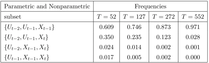
[image:11.595.140.502.330.440.2]with probability one for all i = 1,2, because P(ηt(Ai) = αt) = 0. Thus Assumption A.5 holds. In order to assess both the small and medium sample properties of our theory, we took T = 52 and T = 552. For the four sample sizes of T = 52,127,272 and 552, Table 3.1 gives the relative frequencies of the selected parametric and nonparametric regressors in 1000 replications.
Table 3.1. Frequencies of semiparametric model selection
Parametric and Nonparametric Frequencies
subset T = 52 T = 127 T = 272 T = 552 {Ut−2, Ut−1, Xt−1} 0.609 0.746 0.873 0.971 {Ut−2, Ut−1, Xt} 0.350 0.235 0.123 0.028 {Ut−2, Xt−1, Xt} 0.024 0.014 0.002 0.001 {Ut−1, Xt−1, Xt} 0.017 0.005 0.002 0.000
Remark 3.1. As can be seen from Table 3.1, the true set of regressors {Ut−2, Ut−1, Xt−1}
is selected with increasing frequencies from 0.609 to 0.971 as the sample size increases from
T = 52 to T = 552. The model {Ut−2, Ut−1, Xt}, one of the closest to the true model, is selected with frequencies decreasing from 0.350 to 0.028. This lends support to the efficacy of combining the penalty function method with the leave–one–out cross validation (CV1).
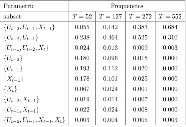
Table 3.2. Frequencies of parametric model selection
Parametric Frequencies
[image:12.595.166.478.152.368.2]subset T = 52 T = 127 T = 272 T = 552 {Ut−2, Ut−1, Xt−1} 0.055 0.142 0.383 0.684 {Ut−2, Ut−1} 0.238 0.464 0.525 0.310 {Ut−1, Ut−2, Xt} 0.024 0.013 0.009 0.003 {Ut−2} 0.180 0.096 0.015 0.000 {Ut−1} 0.193 0.112 0.020 0.000 {Xt−1} 0.178 0.101 0.025 0.000 {Xt} 0.067 0.024 0.001 0.000 {Ut−2, Xt−1} 0.019 0.014 0.007 0.000 {Ut−1, Xt−1} 0.022 0.024 0.008 0.000 {Ut−2, Ut−1, Xt−1, Xt} 0.003 0.004 0.005 0.003
Table 3.3. Frequencies of nonparametric model selection
Nonparametric Frequencies
subset T = 52 T = 127 T = 272 T = 552 {Ut−2, Ut−1, Xt−1} 0.103 0.288 0.464 0.652 {Ut−2, Ut−1, Xt−1, Xt} 0.050 0.103 0.184 0.196 {Ut−2, Ut−1} 0.135 0.205 0.194 0.117 {Ut−2} 0.064 0.022 0.002 0.000 {Ut−1} 0.102 0.035 0.004 0.000 {Xt−1} 0.102 0.048 0.008 0.000 {Xt} 0.059 0.011 0.000 0.000 {Ut−2, Xt−1} 0.053 0.028 0.009 0.000 {Ut−1, Xt−1} 0.058 0.060 0.014 0.002 {Ut−1, Ut−2, Xt} 0.038 0.019 0.092 0.001
new efficient selection method for problems that cannot be solved using existing selection methods for either completely linear models or fully nonparametric models.
The above simulations are based on the assumption that the true model is a partial linear model, for which our method is designed. If the true model is either a parametric model or a fully nonparametric model, our method performs reasonably well. Example 3.2 below considers the case where the true model is a parametric linear model and then applies both the parametric selection proposed by Zheng and Loh (1995) and our own semiparametric selection procedure. When using the proposed semiparametric selection method, our pre-liminary computation suggests involving the same kernel function and bandwidth interval as used in Example 3.1 for the simulation in Example 3.2 below.
Example 3.2. Consider a linear time series model of the form Yt= 0.47Ut−1−0.45Ut−2+
0.5Xt−1 +et, where Ut = 0.55Ut−1−0.12Ut−2 +δt and Xt = 0.3 sin(2πXt−1) +ǫt, in which
δt, ǫt and et are mutually independent and identically distributed as uniform (−1,1), uni-form (−0.5,0.5) and N(0,1), respectively, U1, U2, X1, X2 are independent and identically
distributed as uniform (−1,1), Us and Xt are mutually independent for alls, t ≥3, and the processes{(δt, ǫt, et) :t≥3} are independent of both (U1, U2) and (X1, X2).
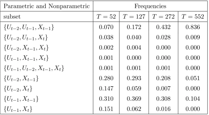
[image:13.595.141.502.522.720.2]ForT = 52,127,272 and 552, we chose the penalty function ΛT(A, D) = (|A|+|D|)T0.5 and then calculated the relative frequencies of the selected parametric and semiparametric regressors in 1000 replications. The results are in Tables 3.4 and 3.5.
Table 3.4. Frequencies of semiparametric model selection
Parametric and Nonparametric Frequencies
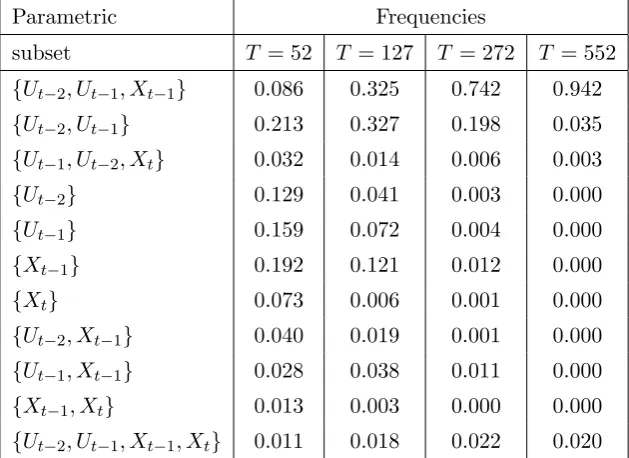
Table 3.5. Frequencies of parametric model selection
Parametric Frequencies
subset T = 52 T = 127 T = 272 T = 552 {Ut−2, Ut−1, Xt−1} 0.086 0.325 0.742 0.942 {Ut−2, Ut−1} 0.213 0.327 0.198 0.035 {Ut−1, Ut−2, Xt} 0.032 0.014 0.006 0.003 {Ut−2} 0.129 0.041 0.003 0.000 {Ut−1} 0.159 0.072 0.004 0.000 {Xt−1} 0.192 0.121 0.012 0.000 {Xt} 0.073 0.006 0.001 0.000 {Ut−2, Xt−1} 0.040 0.019 0.001 0.000 {Ut−1, Xt−1} 0.028 0.038 0.011 0.000 {Xt−1, Xt} 0.013 0.003 0.000 0.000 {Ut−2, Ut−1, Xt−1, Xt} 0.011 0.018 0.022 0.020
Remark 3.3. Tables 3.2 and 3.4 show that semiparametric penalty function method has a similar performance to that of the parametric penalty function method for the cases of
T = 52, T = 127 and T = 272. WhenT = 552, the semiparametric penalty function method does better.
Acknowledgments
The authors would like to thank the Co–Editors, the Guest Editors, and the referees for their constructive comments and suggestions on earlier versions of this paper. Thanks also go to the Australian Research Council Discovery Grants Program for its financial support.
Appendix
There are several basic assumptions stated here. Throughout this appendix, letC(0< C <∞) denote a constant which may have different values at each appearance.
Assumption A.2. For every D∈ D, KD is a |D|-dimensional symmetric, Lipschitz continuous probability kernel function withR kuk2KD(u)du <∞,andKD has an absolutely integrable Fourier transform, wherek · k denote the Euclidean norm.
Assumption A.3. Let Sw be a compact subset of Rq, w(x) be a weight function supported on Sw with 0 < w(x) ≤C for some constant C. For every D ∈ D, let RX,D ⊂ R|D| = (−∞,∞)|D| be the subset such thatXtD ∈ RX,D and letSD be the projection of Sw inRX,D (that is, SD =
RX,D∩Sw). Assume that the marginal density function,fD(·), ofXtD, and the first two derivatives
offD(x), ϕ1(x;D) andϕ2(x;A, D), are all continuous onx∈RX,D, and onSD the density function fD(x) is bounded below byCDand above byCD−1for someCD >0, whereϕ1(x;D) =E[Yt|XtD =x] andϕ2(x;A, D) =E[UtA|XtD=x] for everyA∈ Aand D∈ D.
Assumption A.4. There exists constants 0< C1, C2<∞ such that for any integerl≥1,
sup
x A∈Asup,D∈D
E|Yt−E[Yt|(UtA, XtD)]|l|XtD =x
≤C1, sup
x A∈Asup,D∈D
EkUtAkl|XtD =x
≤C2.
Assumption A.5. For
ηt(A, D) =UtA−E[UtA|XtD], η(A, D) = (η1(A, D),· · ·, ηT(A, D))τ,
ηt=Ut−E[Ut|Xt], η= (η1,· · ·, ηT)τ, Q(A, D) =η(A, D) (η(A, D)τη(A, D))+η(A, D)τ,
and P1T(A, D) = T1(ηβ)τ[IT −Q(A, D)](ηβ), assume that for any given A ∈ A1 and D ∈ D, lim infT→∞P1T(A, D)>0 in probability.
Assumptions A.1–A.5 are standard conditions in this kind of problem. Remark A.1 of Gao and Tong (2002) gives detailed justification for Assumptions A.1–A.5.
To prove Theorem 2.1, the following lemmas are required. Similar to Lemma B.1 of Gao and Tong (2004) and Lemma B.3 of Gao and Tong (2002), we have Lemmas A.1 and A.2. In addition, we include Lemma A.3 to ensure that (2.9) holds.
Lemma A.1 (i) Assume that the conditions of Theorem 2.1 hold. If A ∈ A1 and D ∈ D, then
there existsR1T ≥0 such that
RSS(A, D;h) = T
X
t=1
e2t +T ·P1T(A, D) +T·N1T(D, h) +R1T +oP(T) (A.1)
uniformly inh∈HT D, where R1T is independent of(A, D), P1T is as defined in Assumption A.5,
and
N1T(D, h) =
c1(D)T h1|D| +c2(D)h4+op
1 T h|D|
+op(h4) ifD∈ D1 and h∈HT D,
Here bothc1(D) and c2(D) are positive constants depending on D∈ D1.
(ii)Assume that the conditions of Theorem 2.1 hold. If A∈ A2 and D∈ D, then
RSS(A, D;h) = T
X
t=1
e2t +dAσ2+T ·N1T(D, h) +op(1) (A.2)
uniformly inh∈HT D, where N1T(D, h) is defined as above.
Similar to the proof of Lemma 1(a) of Gao and Tong (2004), it may be shown that for each
givenD, there exist some positive constants d1(D) and d2(D) such that ¯hD =d1(D)T−
1 4+|D| and
N1T(D,¯hD) = min h∈HT D
N1T(D, h) =
d2(D)T−4+4|D| +o
p
T−4+4|D|
, ifD∈ D1,
E{E[Yt|XtD]−E[Yt|Xt]}2+op(1), ifD /∈ D1.
(A.3)
Lemma A.2. Assume that the conditions of Theorem 2.1 hold. If A∈ A1 and D∈ D then
lim inf
T→∞ Q1T(A, D) = lim infT→∞ P1T(A, D)>0 in probability, (A.4)
where Q1T(A, D) = T1(V β)τR(A, D)(V β), P1T(A, D) and R(A, D) are defined as before.
Lemma A.3. Assume that the conditions of Theorem 2.1 hold. Then, uniformly in h∈HT D,
RSS(A, D;h) =ετR(A, D)ε+ ˜Φ(D)τR(A, D) ˜Φ(D) + (V β)τR(A, D)(V β) +oP(RSS(A, D;h)), (A.5)
MT(A, D;h) =E[RSS(A, D;h)] = (T− |A|)σ2+PT(A, D) +NT(A, D) +o(MT(A, D;h)). (A.6)
Proof: Write
∆T(A, D;h) = 2ετR(A, D) ˜Φ(D) + 2 ˜Φτ(D)R(A, D)(V β) + 2ετR(A, D)(V β). (A.7)
In order to prove (A.5), it suffices to show that for sufficiently largeT
sup h∈HT D
|∆T(A, D;h)|
RSS(A, D;h) =oP(1), (A.8)
which follows from
sup h∈HT D
ετR(A, D) ˜Φ(D)
RSS(A, D;h) =oP(1), h∈supHT D
Φ˜τ(D)R(A, D)(V β)
RSS(A, D;h) =oP(1), (A.9)
sup h∈HT D
|ετR(A, D)(V β)|
The proofs of (A.9) and (A.10) are quite standard in this kind of problem. The details are as in the proof of (A.18) of Gao and Yee (2000) for example, and are omitted here. The proof of (A.6) follows from (A.5) using the Dominated Convergence Theorem.
Proof of Theorem 2.1: Let RSS(A, D) = minh∈HT DRSS(A, D;h). In view of (A.1)–(A.3), we
can writeRSS(A, D) as
RSS(A, D) =
PT
t=1e2t +T ·P1T(A, D) +T·N1T(D,¯hD) +R1T +op(T) A∈ A1, D∈ D,
PT
t=1e2t +dAσ2+T·N1T(D,¯hD) +op(1) A∈ A2, D∈ D.
It follows immediately fromP1T(A∗, D∗) = 0 that RSS(A, D)−RSS(A∗, D∗)
=
T ·P1T(A, D)−dA∗σ2+T(N1T(D,¯hD)−N1T(D∗,¯hD∗)) +op(T) A∈ A1, D∈ D,
(dA−dA∗)σ2+T(N1T(D,h¯D)−N1T(D∗,h¯D∗)) +op(1) A∈ A2, D∈ D.
IfA∈ A2 and D∈ D, then asT → ∞,
1−PRSS(A, D)−RSS(A∗, D∗) + (ΛT(A, D)−ΛT(A∗, D∗))bσ2>0
=P(dA−dA∗)σ2+T(N
1T(D,¯hD)−N1T(D∗,¯hD∗)) +op(1) + (ΛT(A, D)−ΛT(A∗, D∗))σb2≤0
=P
N1T(D,¯hD)−N1T(D∗,hD¯ ∗)≤ −
dA−dA∗
T σ
2−ΛT(A, D)−ΛT(A∗, D∗)
T bσ
2
≤P
N1T(D,¯hD)−N1T(D∗,hD¯ ∗)≤ −
dA−dA∗
T σ
2−ΛT(A, D) T
1−ΛT(A∗, D∗)
ΛT(A, D)
·1
2σ 2
+o(1)
≤P
N1T(D,¯hD)−N1T(D∗,¯hD∗)≤ −
ΛT(A, D) T
1−ΛT(A∗, D∗)
ΛT(A, D)
·1
2σ 2
+o(1)→0 (A.11)
because ofN1T(D,¯hD)−N1T(D∗,¯hD∗)>0 for allA∈ A1 and eitherD∈ D1 orD∈ D − D1.
IfA∈ A1 and D∈ D, then we obtain asT → ∞,
1−PRSS(A, D)−RSS(A∗, D∗) + (ΛT(A, D)−ΛT(A∗, D∗))bσ2>0
=P
P1T(A, D) + N1T(D,¯hD)−N1T(D∗,¯hD∗)
+R1T−dA∗σ
2+ (ΛT(A, D)−ΛT(A
∗, D∗))bσ2
T +oP(1)≤0
=P
P1T(A, D) +N1T(D,¯hD)−N1T(D∗,hD¯ ∗)≤ −
op(T)
T +
dA∗σ
2
T −
R1T
T −
(ΛT(A, D)−ΛT(A∗, D∗))σb2
T
+o(1) =P
P1T(A, D) +N1T(D,¯hD)−N1T(D∗,¯hD∗)≤ −
ΛT(A, D) T
1−ΛT(A∗, D∗)
ΛT(A, D)
· 1
2σ 2
+o(1)→0 (A.12)
because of lim infT→∞P1T(A, D) > 0 and N1T(D,¯hD)−N1T(D∗,¯hD∗) > 0 for all D ∈ D1 or
Consequently, as T → ∞,
1≥P( ˆA=A∗,Dˆ =D∗)≥PnRSS(A, D)−RSS(A∗, D∗) + (ΛT(A, D)−ΛT(A∗, D∗))σb2 >0
o
→1.
This completes the proof of the first part of Theorem 2.1. Now if ˆh= ¯hDˆ,c∗ =cD∗ andh∗ = ¯hD∗=
c∗T−4+|1D∗|, it follows from the above proof and (A.3) that ˆh
h∗ →p1 asT → ∞. This completes the
proofs.
References
Akaike, H. (1973). Information theory and an extension of the maximum likelihood principle. In 2nd International Symposium on Information Theory (Edited by B. N. Petrov and F. Cs´aki), 267–281. Akad´emiai Kiado, Budapest.
Cheng, B. and Tong, H.(1992). On consistent nonparametric order determination and chaos. J. Roy. Statist. Soc. Ser. B 54, 427–449.
Gao, J. and Tong, H.(2002). Nonparametric and semiparametric regression model selection. Working paper available from www.maths.uwa.edu.au/˜jiti/kao43.pdf.
Gao, J. and Tong, H. (2004). Semiparametric nonlinear time series model selection. J. Roy. Statist. Soc. Ser. B 66, 321–336.
Gao, J. and Yee, T. (2000). Adaptive estimation in partially linear (semiparametric) autoregressive models. Canad. J. Statist. 28, 571–586.
H¨ardle, W., Hall, P. and Marron, J.(2002). Regression smoothing parameters that are not far from their optimum. J. Amer. Statist. Assoc. 87, 227–233.
Mallows, C. L. (1973). Some comments onCp. Technometrics15, 661–675.
Masry, E. and Tjøstheim, D.(1995). Nonparametric estimation and identification of nonlinear ARCH time series. Econometric Theory11, 258–289.
Masry, E. and Tjøstheim, D. (1997). Additive nonlinear ARX time series and projection estimates.
Econometric Theory13, 214–252.
Shao, J. (1993) Linear model selection by cross–validation. J. Amer. Statist. Assoc. 422, 486–494.
Shibata, R. (1976). Selection of the order of an autoregressive model by Akaike’s information criterion.
Biometrika 63, 117–126.
Yao, Q. and Tong, H. (1994). On subset selection in nonparametric stochastic regression. Statistica Sinica4, 51–70.
Zhang, P. (1993). Model selection via multifold cross–validation. Ann. Statist. 21, 299–313.
Zheng, X. and Loh, W. Y. (1995). Consistent variable selection in linear models. J. Amer. Statist. Assoc. 90, 151–156.
Zheng, X. and Loh, W. Y. (1997). A consistent variable selection criterion for linear models with high–dimensional covariates. Statistica Sinica7, 311–325.
Department of Applied Mathematics, Shanxi University of Economics and Finance, P. R. China [email protected]
School of Mathematics and Statistics, The University of Western Australia, Australia [email protected]