A Simple Approach to SQL Joins in a Relational Algebraic Notation

(1)

A Simple Approach to SQL Joins in a Relational

Algebraic Notation

C.Bhanuprakash

Assistant Professor, Dept.of MCA, SIT Tumkur – 572103,Karnataka.

Y.S.Nijagunarya

, PhD

Professor,

Dept.of CSc and Engg, SIT Tumkur-572103, Karnataka.

M.A.Jayaram

, PhD

Professor, Dept.of MCA, SIT Tumkur – 572103, Karnataka

ABSTRACT

Join is an operation in accessing the data from table if number of tables exceeds one. Whenever we need the data which is not available from a single table, then it needs to necessitate using join operation. Sometimes join is required even if there is a single table. It all depends on the format in which we need to display the data in the user environment.

In join processes, the accessing of the data depends on the joining conditions with different operators. Here, join condition is a must. For this purpose, generally we are using relational operators along with logical operators. The problem presently we are facing is many of them are not knowing exactly all types of joins, their proper syntaxes and their proper usage. Sometimes it is vey difficult for the teacher or trainer to convince the trainees, students, research scholars in giving right practical examples while we teach SQL joins to them. Even if we use some conventional operators, the performance of the query may results in delayed accessing time in retrieving the data from N number of tables. This is due to lack of knowledge of the programmers on evaluation criteria of the joined queries. Since the present tables are dealing with millions of records, if we take these tables as example tables, then it is very difficult to give the exact demonstration regarding the number of records to be accessed, because, many joining concepts dealing with exact number of records which are working based on Cartesian Product. To avoid all these uncertainties, confusion, ambiguities, in this paper, it has been used with only three simple tables which are given from Oracle Corporation in user schema scott/tiger. The number of records used in these tables is very minimum and are meaningful records.

After understanding the basics of all SQL joins, then it is necessary to represent the same queries in relational algebraic notations, because, those are the standard and uniform syntaxes which will be applicable in any of the database software. But the present problem is many of the software developers, specialists, programmers, and researchers are not aware of how to represent queries exactly in that syntax. In order to overcome this, the main focus is to make a familiarity in writing the SQL queries in relational algebraic format along with different types of joins.

The main focus of this paper is to learn the basic fundamentals of all types of SQL joins along with algebraic notations in a very easiest, convinced and simple approach. On many stages, it is given with live examples along with SQL code and its result set by using SQLPLUS interface.

General Terms

In this paper, records of the table are referred as result set and the records which are matching the joining condition are referred as matching records.

Keywords

SQL Joins, Relational operators, Relational Algebraic expressions, Query evaluation, Access time, matching records, Result set.

1. INTRODUCTION

A join is a query that combines data records from two or more tables. We perform a join whenever multiple tables appear in the FROM clause of the query. We can specify any number of columns of the table in the select clause of the query. Then find out the common column from both the tables for framing the join condition along with some relational operator, preferably always with equal operator (=). If any two of these tables have a common column name, then we refer these columns throughout the query with table name as primary identifier to avoid ambiguity (Example : Emp.Deptno).

The basic set of operations to manipulate the relational model is the relational algebra. These operations familiarize the user to specify basic retrieval requests. The result of a retrieval is always becomes the new relation [1], that may be formed from one or more relations. The algebra operations thus produce new relations which can be further manipulated using the same algebraic operations. A sequence of relational algebra operations forms a relational algebra expression, whose result will also be a relation that represents the result of a database query. The relational algebra is very important for several reasons.



It provides a proper and basic foundation for relational model operations.



It is used as a basic template for implementing and optimizing queries in RDBMS



Some of its concepts are used in SQL.

Presently, even though no RDBMS software is providing an interface for relational algebra queries, the core operations and functions of any relational system are based on relational algebra operations only.

1.1 Joining conditions

(2)

the join conditions need not be appear in the select list. It is an optional one.

To execute a join of three or more tables, SQL engine first joins two of the tables based on the join conditions comparing their columns and then joins the result to another table based on join conditions containing columns of the joined tables and the new table. SQL engine continues this process until all tables are joined into the result. The optimizer specifies the order in which SQL engine joins tables based on the join conditions, indexes on the tables, and, any available statistics for the tables [1].

In addition to join conditions, the WHERE clause of a join query can also contain other conditions that refer to columns of only one table. These conditions can further filter the records returned by the join query.

2. TYPES OF JOINS

Mainly there are three types of joins based on the way they retrieve the records. They are Inner join, Outer join and joining more than two tables.

2.1 Inner Join :

An inner join (sometimes called a

simple join) is a join of two or more tables that returns only those records that satisfy the join condition. I.e. it is looking for only the matching records [1].

( What is a Matching record ? It is the one which satisfies the joining condition. I.e. its existence and relationship will be there in both the tables.)

2.2 Outer Join :

An outer join extends the result of a simple join. An outer join returns all records that satisfy the join condition and also returns some or all of those records from one table for which no record from the other table satisfy the join condition. In other words, first of all it is looking for matching records and remaining records (usually with null values) from one table or both the tables [1].

2.3 Joining more than Two tables :

It is a generalized joining process in which number of tables is exceeding by two. Here, the minimum number of joining conditions required depends on the number of tables being joined. To join N number of tables, at minimum, we need (N – 1) joining conditions [4].

3. RELATIONAL OPERATIONS

3.1 The PROJECT operation :

It selects certain columns from the table and discards the remaining columns. If we want to retrieve only certain attributes of a relation or all the attributes, we use the PROJECT operation.[6] The general form of the PROJECT operation is

π

< attribute list>

(R)

Here, π is the symbol used to represent Projection, <attribute list> is the list of columns (attributes) of a relation R and (R) is the relation name (table name)

3.2 The SELECT operation :

It is used to select a subset of the records from a relation that satisfies a select condition. It acts like a filter by selecting only required records by putting the condition in a query [7]. The general form of the SELECT operation is

σ

< select condition>

(R)

The Boolean condition specified in <select condition> is made up of a number of clauses of the form

Here, attribute name is column name, comparison operator is equal operator ‘=’ and constant value is a user defined value.

3.3 The JOIN operation :

It is used to combine related records from one, two or more relations in to a single record [8]. A general form of JOIN operation on two relations is

R

<join condition> S

Here R is the first relation, S is the second relation, <join condition> contains R.Column=S.Column R and S are the two relations, Column is the common column available from both the relations.

If number conditions increases, then conditions will be included by using Logical operators (i.e. AND, OR, NOT)

3.4 Cartesian Product :

If two tables in a join query have no join condition, then query results in a type of a result set in the form of Cartesian product. Query combines each row of one table with each row of the other [5]. It is in the form of M X N. i.e. M is the number of records in first table and N is the number of records in the second table [4]. A Cartesian product always generates many rows and is rarely useful. For example, the Cartesian product of two tables, each with 50 rows, has 2,500 rows. Therefore always be careful in using join conditions. If a query joins three or more tables and you do not specify a join condition for a specific pair, then the optimizer may choose a join order that avoids producing an intermediate Cartesian product.

4. PRACTICAL APPROACH

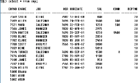
To explain all the above joining types, here it is used with following tables which are available from Oracle software under user schema scott/tiger. Their structures and records are shown in Table-EMP.

Table-EMP (Table description)

(3)

Table. : EMP ( Table with records )

Table : DEPT ( Table description)

[image:3.595.55.286.99.238.2]

This table with the name “DEPT” will keep track of the data of the different departments regarding the department Id, department Name and its location in an organization. In this table, the column DEPTNO is the primary key. Since we do not have any foreign key in this table, we consider this table as MASTER TABLE. There are 7 records in this table. Its records are displaying as shown in Table - DEPT.

Table – DEPT. ( Table with records )

Table – 3 : SALGRADE ( Table description )

[image:3.595.316.499.206.279.2]

This table with the name “SALGRADE” will keep track of the data of the salary grades maintaining in an organization in the form of Grade, staring salary limit, upper salary limit. In this table, we do not have any primary key or foreign key, we consider this table as a general table . There are 5 records in this table. Its records are shown below. We will be using this table when we need the grade of an employee based on the salary he is getting.

Table – SALGRADE (Table with records)

4.1 INNER JOIN :

As mentioned earlier, this join will mainly looking for matching records. i.e. the records which satisfy the joining condition [3]. There are three types in this inner join. They are

a) Inner Equi join, b) Inner Non-Equi join c) Inner Self join

4.1.a. Inner Equi-Join :

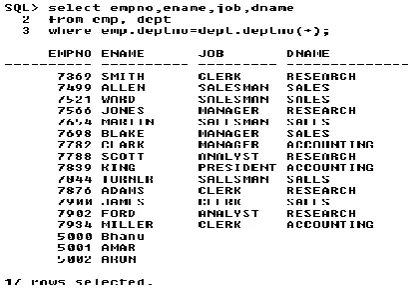
An equijoin is a join with a join condition containing an equality operator [2]. An equijoin combines records that have equivalent values for the specified columns. Depending on the implicit algorithmic plan, the optimizer chooses the execution plan for this equijoin. The size of the columns specified in the joining condition in a table may be restricted to the size of a data block without some overheads. The size of a data block is specified by the initialization parameter DB_BLOCK_SIZE [1].

To give an example to this join, here it is used with EMP and DEPT tables. This join needs one common column. i.e. DEPTNO which acts as Primary key in DEPT table and Foreign key in EMP table. The joining condition requires the usage of EQUAL operator. The following SQL query retrieves the employee number, employee name, designation and department name from the tables EMP and DEPT

Example : SQL>select empno,ename,job,dname From emp, dept

Where emp.deptno=dept.deptno;

Relational Algebra notation :

[image:3.595.55.267.515.610.2]

(4)

Result



π <

empno,ename,job,dname

>(

emp

<

deptno=deptno

>)

dept

or it can also be represented as

R1



π <

>

emp,dept

R2



emp < deptno=deptno> dept

The resultant result is given by

R  R1(R2)

After execution, the query will get only 14 matching records. i.e. records which satisfies the joining condition.

4.1.b Inner Non Equijoin

:

A Non equijoin is a join with a join condition without containing an equality operator. A non-equijoin combines records that have equivalent values for the specified columns. Depending on the implicit algorithmic plan the optimizer chooses the execution plan for this join [3].

To give an example to this join, here it is used with EMP and SALGRADE tables. This join does not require any common column or master child relationship among the tables. The joining condition prohibits the usage of EQUAL operator. The following SQL query retrieves the employee number, employee name, salary and grade from the tables EMP and SALGRADE.

Example : SQL>select empno,ename,sal,grade From emp, salgrade

Where sal>=losal and sal <= hisal;

Result



π <

empno,ename,sal,grade

>(

emp

<

sal

=>

losal AND sal

<=

hisal

>)

salgrade

R1



π <

empno,ename,sal,grade

>

emp, salgrade

R2



emp _{< sal >= losal AND sal <= hisal>}salgrade

R  R1(R2)

After execution, the query will get only 14 matching records. i.e. records which satisfies the join condition.

This can also be executed by using one more operator “BETWEEN”

Example : SQL>select empno,ename,sal,grade From emp, salgrade

Where sal between losal and hisal;

Note : be careful in using BETWEEN operator, i.e. the first parameter value should be less than second parameter.

4.1.c Inner Self Join :

A self-join is a join of a table to itself. Since a join requires minimum of two tables, here, we refer the same table twice in the FROM clause and is followed by table aliases that qualify column names in the join condition. To perform a self-join, oracle combines and retrieves records of the table that satisfy the join condition [3].

To give an example to this join, here it is used with EMP table only. In this table, the column EMPNO is primary key and MGR is foreign key which references primary key of the same table. This join is the concept works under the UNARY relationship. The following SQL query retrieves the employee name in one column and their respective managers in the other column. Here, the same EMP table will be referenced twice with alias name.

Example : SQL>select E.ename as Employee, M.ename as Manager

From emp E, emp M Where M.empno=E.mgr;

Result



π <

E.ename as Employee, M.ename as Manager

>(

E.emp

<

M.empno = E.mgr

>)

M.emp

R1



π <

E.ename as Employee, M.ename as

Manager

>

E.emp,M.emp

R2



E.emp

_<

_{M.empno = E.mgr}

_>

M.emp The resultant result is given by

[image:4.595.57.270.234.383.2]

(5)

After execution, the query will get only 13 matching records. i.e. records which satisfies the join condition. Why only 13 records ? why not 14 as in the case of previous two cases. Here one of the employees with the name ‘KING’ do not have manager. That’s why, it is only 13 records here.

4.2 OUTER JOIN :

As mentioned earlier, this join is an extension of inner join. It is mainly looking for matching records and remaining records from either of the tables or both the tables [2]. There are three types in this outer join. They are

a) Left outer join b) Right outer join c) Full outer join

4.2.a) Left Outer Join :

As the name itself indicates that, this query mainly looking for matching records and remaining records from left table [7]. How do we know that which is left table ? and which is right table ?. It will be decided by looking the following join condition.

Table-A.Column_Id = Table-B.Column_Id(+)

Here, the table which is located at the left hand side of equality operator is considered as Left table and the table specified at the right hand side of equality operator is considered as Right table. In the above case, Table-A is left table and Table-B is right table. There is a provision to use any table in any of the side.

To give an example to this join, here it is used with EMP table as left table and DEPT table as right table. The following SQL query retrieves the records containing the employee number, employee name, designation, and department name in which he is working.

Example : SQL>select empno, ename, job, dname from emp, dept

Where emp.deptno=dept.deptno (+);

Result



π <

>(

emp

<

deptno=deptno

>)

Dept

R1



π <

>

emp, dept

R2



emp _{< deptno=deptno>}dept

R  R1(R2)

After execution, the query will get 17 records. Out which, 14 records are matching records and remaining 3 records are from only left table. i.e. the records with null values in the columns job and dname.

The same query can also be written as follows.

SQL > select empno,ename,job,dname From emp left outer join dept On emp.deptno=dept.deptno;

4.2.b) Right Outer Join :

This join query mainly looking for matching records and remaining records from right table [4].

To give an example to this join, here it is used with EMP table as left table and DEPT table as right table. The following SQL query retrieves the records containing the employee number, employee name, designation, and department name in which he is working.

Example : SQL>select empno,ename,job,dname from emp, dept

Where emp.deptno(+)=dept.deptno;

Result



π <

>(

emp

<

deptno=deptno

>)

Dept

OR it can also be represented as

R1



π <

>

emp, dept

R2



emp < deptno=deptno>dept

R  R1(R2)

[image:5.595.315.524.164.308.2]

(6)

The same query can also be written as follows.

SQL > select empno,ename,job,dname From emp right outer join dept On emp.deptno=dept.deptno;

4.2.c) FULL Outer Join :

This join query mainly looking for matching records and remaining records from both the tables [3].

[image:6.595.53.277.69.263.2]

To give an example to this join, here it is used with EMP table as left table and DEPT table as right table. The following SQL query retrieves the employee number, employee name, designation, and department name in which he is working.

Example : SQL>select empno,ename,job,dname from emp Full outer join dept

on emp.deptno=dept.deptno;

Result



π <

>(

emp

<

deptno=deptno

>)

Dept or it can also be represented as

R1



π <

>

emp, dept

R2



emp < deptno=deptno> dept

R  R1(R2)

After execution, the query will get 21 records. Out which, 14 records are matching records and remaining 3 records are from left table and remaining 4 records from right table.

4.3 Joining more than two tables :

It is a generalized joining process in which number of tables are exceeding by two. Here, the minimum number of joining conditions required depends on the number of tables being joined [4]. To join N number of tables, at minimum, we need (N – 1) joining conditions.

To give an example to this join, here it is used with 5 tables. Namely BRANCH, CLASS, SUBJECT, TEACHER and STUDENT. Their structures and records are as follows :

Table- Branch

This Branch table is a master table which keep tracks of all the branches in a college. Here, the column, BranchId is a primary key.

(7)

This Class table is a master table which keep tracks of all the classes in a college. Here, the column ClassId is a primary key.

Table- Subject

This Subject table is a master table which keep tracks of all the subjects taught in a college. Here, the column SubjectId is a primary key.

Table- Teacher

This Teacher table is a master table which keep tracks of all the Teachers in a college. Here, the column TeacherId is a primary key.

Table- Student

This Student table is a child table which keep tracks of all the students in a college. Here, the column StudentId is a primary key and columns Branchid, ClassId, SubjectId, and TeacherId are foreign keys. i.e. student is the child table having relationship with remaining four tables. If we access the records from student table, the data leads to lot of ambiguities, confusions to the users. They may not know what is branchid, subjectid, classid or teacherid. To avoid this, we will be joining all the above tables to give meaningful data to the users. i.e. to display Branch name, Class name, subject name, teacher name to the users, but all these columns are available from master tables and their id columns are shared with child table. That’s why it needs to join these tables to give meaningful result.

Relational Algebra notation : Here it is a combination of projection and Join.

Result



π <

StudentId, StudentName, BranchName, Classname, Subjectname,

Teachername

>(

Student

<

BranchId=BranchId

>)

Branch

AND

(

Student

<

ClassId=ClassId

>)

Class

AND

(

Student

<

SubjectId=SubjectId

>)

Subject AND

(

Student

<

TeacherId=TeacherId

>)

Teacher or it can also be represented as

R1



π <

StudentId, StudentName,BranchName,

Classname,Subjectname,

Teachername

>

student,Branch,Class,Subject,Teacher

R2



(

Student

<

BranchId=BranchId

>)

Branch

AND

(

Student

<

ClassId=ClassId

>)

Class AND

(

Student

<

SubjectId=SubjectId

>)

Subject AND

(

Student

<

TeacherId=TeacherId

>)

Teacher The resultant result is given by

R  R1(R2)

(8)

needed depends on our requirement. Say for example, If we need the details of the students belongs to only computer science branch, then we need n-1 joining conditions and condition which access the computer science branch students. This is as follows.

Relational Algebra notation : Here it is a combination of Projection, Selection and Join.

Result



π <

Teachername

>(σ<

Branchname=’CompSc’

>)

Branch AND

(

Student

<

BranchId=BranchId

>)

Branch

AND

(

Student

<

ClassId=ClassId

>)

Class AND

(

Student

<

SubjectId=SubjectId

>)

Subject AND

(

Student

<

TeacherId=TeacherId

>)

Teacher

)

R1



π <

StudentId, StudentName, BranchName,

Classname, Subjectname, Teachername

>

R2



σ<

>

Branch

R3



(

Student

<

BranchId=BranchId

>)

Branch

AND

(

Student

<

ClassId=ClassId

>)

Class AND

(

Student

<

SubjectId=SubjectId

>)

Subject AND

(

Student

<

TeacherId=TeacherId

>)

R  R1 (R2 (R3))

In addition to this if we need to access the student details belongs to I semester computer science students then it needs one more additional condition.

Here it is a combination of projection, Selection and Join.

Result



π <

Teachername

>(σ<

Branchname=’CompSc’ AND <ClassName=’I Sem’

>)

Branch

AND

(

Student

<

BranchId=BranchId

>)

Branch

AND

(

Student

<

ClassId=ClassId

>)

Class AND

(

Student

<

SubjectId=SubjectId

>)

Subject AND

(

Student

<

TeacherId=TeacherId

>)

Teacher

)

R1



π <

StudentId, StudentName, BranchName,

Classname, Subjectname,

Teachername

>

R2



σ<

AND ClassName=’I Sem’

>

Branch R3



(

Student

<

BranchId=BranchId

>)

Branch

AND

(

Student

<

ClassId=ClassId

>)

Class AND

(

Student

<

SubjectId=SubjectId

>)

Subject AND

(

Student

<

TeacherId=TeacherId

>)

R  R1 (R2 (R3))

Like these, if more number of tables to be joined with varied type of requirements, then complexity in making the joining conditions may also increases. But it needs basic knowledge on SQL queries with proper syntaxes and skills in arranging the conditions. Thorough working on different queries with varied requirements will make you more perfect in framing the SQL statements in more effective ways.

5. CONCLUSION AND FUTURE WORK

In this paper, the concept of different SQL joins has been explained by giving simple examples along with their respective relational algebraic notations. These notations are applied on simple database tables for easy understanding and also to accessing the data set from different tables in an easiest way. While doing so, the difficulty in learning some of the complex joins has been minimized. It is mainly focused on how to write relational algebraic notation by splitting into smaller result sets and then combine them to become resultant result. This is simply to understand in a step by step by approach in case of complex join conditions. But still lot of scope will be there to make lot of research in this regard to enhance the performance level of the join queries to the optimized extent.

To explain these concepts effectively to the trainees, scholars and students, here it is taken with simple generalized tables which were given by Oracle Corporation with less number of records with user schema scott/tiger (username as “scott” and “tiger” as password). To work with these SQL join queries practically, it is suggesting to use oracle software with minimum version of 9i onwards.

(9)

6. REFERENCES

[1] Oracle® Database SQL Reference 10g Release 1 (10.1), Documentation.

[2] Fundamentals of Database Systems, Fifth Edition, by Ramez Elmasri, Shamkant B.Navathe, Pearson Publications, 2009.

[3] Database Management Systems, By – Raghuramakrishnan, Gehrke, Third Edition, McGraw-Hill Publications, 2003.

[4] Pratt, Phillip J (2005), A Guide To SQL, Seventh Edition, Thomson Course Technology, ISBN 978-0-619-21674-0

[5] Shah, Nilesh (2005) [2002], Database Systems Using Oracle – A Simplified Guide to SQL and PL/SQL Second

Edition (International ed.), Pearson Education International, ISBN 0-13-191180-5

[6] Yu, Clement T.; Meng, Weiyi (1998), Principles of Database Query Processing for Advanced Applications, Morgan Kaufmann, ISBN 978-1-55860-434-6, retrieved 2009-03-03

[7] M. Tamer Özsu; Patrick Valduriez (2011). Principles of Distributed Database Systems (3rd ed.). Springer. p. 46. ISBN 978-1-4419-8833-1.