An Efficient Gradient based Algorithm for Improving Performance of Image Edge Detection

An Efficient Gradient based Algorithm for Improving

Performance of Image Edge Detection

Majid Reza Vahidi

Department of Engineering, North Tehran branch, Islamic Azad University, Tehran, Iran

Mohammad Mansour

Riahi Kashani

Department of Engineering, North Tehran branch, Islamic Azad University, Tehran, Iran

Alireza Bagheri

ABSTRACT

Quality and execution time are two important factors for evaluation of edge detection algorithms. In these algorithms, there is a trade-off between quality and execution time. Some algorithms only concentrate on quality and some of them are fast and low quality. Efficient methods try to achieve high quality in a low time. This research concentrates on improvement of gradient based edge detection that is fast method and appropriate for real-time processing. The proposed algorithm reduces execution time by removing many pixels from computations. It calculates gradient and angle class of remaining pixels in a very efficient way so that it reinforces quality and locality of edges. The results of this algorithm indicated improvement of performance in comparison to Canny and LOG algorithms.

General Terms

Computer Vision, Image segmentation, Edge detection.

Keywords

Edge detection algorithm, Gradient of image, Angle Class of pixel, Non-Maximum Suppression, Post reduction of noise, Edge detector evaluation, Locality of edges, Quality of edges.

1.

INTRODUCTION

Edge detection in images has been considered from the beginning of image processing and machine vision history. Edges can be defined as boundaries between objects or boundaries between objects and background image and are represented by continuous lines and curves.

The main reason of using edge detection is to exploit its output for next further processing. After this pre-processing, an image is extracted containing only important information of main image. Therefore, inconsiderable information of main image is removed so that firstly the processing effort and execution time are reduced and secondly the content of image can be processed by the algorithms which operate only on lines and curves.

In researches based on cellular learning automata [1-2] performance measures have not been considered and the focus has been on the quality of edges. In Methods based on cellular automata [3-4] execution time has not been considered. Methods based on Morphology [5-6] need many computations for gray scale images. Furthermore methods based on wavelet [7-8] have multiple scales and need to measure Lipschitz regularity, that makes them time consuming.

Gradient based algorithms are fast and appropriate for real-time processing. In addition to gradient based algorithms, many other algorithms use gradient values to achieve better

parametric membership functions to transform the gradients into fuzzy membership degrees for edge detection. Canny presented a gradient based algorithm for edge detection [14] that has been the base for many researches. In recent years, improvements have been made on it. One of the improved versions of Canny’s algorithm was specially designed for images distorted by Gaussian noise [15]. Another improved version of Canny’s algorithm based on type-2 fuzzy sets operates better in vague region boundaries [16]. Also [17] proposed a new fusion algorithm based on wavelet transform and Canny operator to detect image edges. Although Canny’s algorithm achieves good quality, its execution is time-consuming. Unfortunately in edge detection, there is a trade-off between quality and execution time.

Quality in edge detection is quite important. Extraction of blurred, broken or thick edges makes the following processing steps difficult. That is why one of researches’ aims has been to find ways that can help obtain high quality edges in a smaller amount of time. This research’s purpose is to obtain the same results.

The proposed algorithm does not suffer from some practical limitations [18] of gradient based edge detection. In the proposed algorithm, image is smoothed by a small filter and remaining noise is removed after edge detection. Also calculating gradient is different from that in Sobel and Prewitt methods. These operators generally calculate gradient by combining horizontal and vertical directions while in the proposed algorithm, maximum of gradients is calculated regarding horizontal, vertical and diagonal directions. Although in this quality related step, the number of comparisons in each pixel is at most eight, not checking the pixels which are brighter than average value of their neighboring pixels in the following steps, reduces processing effort and execution time. In common implementation of Canny’s algorithm, for finding direction of each pixel, tangent is calculated and angle of pixel is determined and then the angle class is used. Due to the fact that calculating Arctangent takes time, in this algorithm instead of calculating angle of each pixel, angle class is determined directly. Finally, angle class is used for Non-Maximum suppression that leads to thin edges. In Canny’s algorithm Non-Maximum suppression is run on all the pixels of image while in the proposed algorithm, this process is only run on the remaining edges.

Eventually in this algorithm, post processing is run on extracted edge image. In post processing step of Canny’s algorithm, edge restoration is done while in the proposed algorithm, remaining noise is removed. That is done by considering the isolated pixels which do not have a path to other edge pixels.

Department of Computer Engineering and IT, Amirkabir University of

2.

STEPS OF THE PROPOSED

ALGORITHM

2.1

Smoothing and computational

complexity

First step of gradient based edge detection is to remove noise. Gaussian filter uses n×n mask where n is an odd value and must be equal to three or greater. Not only do high n values lead to edge displacements and faded edges, but they also increase running cost. So, smallest n can be considered. For example, for the average filter (3×3), no multiplication, only eight summations and one division are required. Considering less computation in these filters, at the first step of this algorithm, a small filter is used and remaining noises are removed in the “Post reduction of noise” step.

2.2

Average of neighborhood

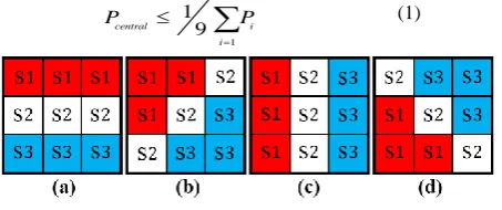
This step is one of the key parts of this algorithm which reduces the execution time. Assuming existence of edge environs the central pixel, if the value of central pixel is higher (brighter) than the average value of its neighboring pixels, the central pixel cannot be an edge, because there are pixel(s) in the neighborhood of this pixel, which are boundary of intensity; so there is no necessity to carry out calculations on the central pixel. The proposed algorithm limits calculations to the pixels which are darker or equal to average of their neighboring pixels that leads to reduce the processing effort. Pixels which match the equation 1 are selected for the next steps. 9 1 1 9 central i i P P 





Fig 1: Determining gradient value and angle class. Angle class of: a) zero and 180, b) 45 and 225, c) 90 and 270, d)

135 and 315 degrees

2.3

Thresholding and calculating gradient

value

Steps 2.3 and 2.4 are mixed to reduce the processing effort. The part of algorithm (Algorithm 1) indicates that the proposed algorithm does not use blind convolution on whole image. In the proposed algorithm, neighborhood of 3×3 pixels are considered and followed by determining that the pixel is darker or equal to the average value of its neighboring pixels, at most eight directions of the pixel are checked. For each direction, the value of summed pixels is subtracted from the opposite side’s summed pixels. If this value is upper than threshold, the pixel is recognized as primary edge.

Figure 1 shows summed pixels with the same set. For calculating gradient in each of these eight directions, summed pixels of s1 or s3 minus summed pixels of s2 is considered as the gradient value of that direction (equation 2).

i k n i j

P P ThresholdGradient  P P

 

 

1, 2, 3, 1 8

3, 2, 1, 1 8

i j k

i j k

P S P S P S n OR

P S P S P S n

      

    



2.4

Finding the direction of gradient

Angle class is used for grouping angles of pixels. There is a gradient value for each angle class in Figure1. For each of them in Figure1, gradient value of angle class is compared to the maximum gradient value of its previous angle classes, and maximum value is assigned to main gradient (equation 3) and along with it, main angle class of pixel is determined. In each direction that a gradient value has been detected to have a maximum, its direction is assigned to angle class of central pixel (equation 4).





GMax G G G n (3)

C()C( _G) (4)

Calculating gradients in at most eight directions can map the status of central pixel to one of the angle classes like shown in Figure 2. For example, in Figure 1b, if s1s minus s2s is maximum among other directions (Figure 1 a, b, c, d), it means that in gray scale image, values of s1 region are brighter than values of s3 region; and according to the dominance of this direction to other directions, this status can be mapped to Figure 2 which its angle class is 45 degree. Algorithm 1 (2.3 And 2.4)

Main gradient =0;

For each of the states (a, b, c, d) in Figure 1{ If (difference of neighborhood> Threshold) { Mark pixel as primary edge;

If (gradient of angle class > main gradient) {main gradient= gradient of angle class; main angle class= this angle class ;}

}

Else if (difference of neighborhood< - Threshold) { Mark pixel as primary edge;

If (gradient of opposite angle class > Main gradient) {main gradient =gradient of opposite angle class; main

angle class = opposite angle class ;} }

}

Fig 2: 45 degree class

Fig 3: Selecting the pixel for comparing to the central pixel based on angle class

2.6

Post reduction of noise

Now, edges are obtained with one pixel width and it is likely that there are pixels in image which are not along the edges. This is related to selecting threshold. When a threshold is lower than its proper value, although more edges are obtained, noisy points increase. In fact, this step is designed for making flexibility to select threshold and also completing the smoothing step of this algorithm.

Fig 4: Post reduction of noise. a) The pattern which is removed, b) The pattern which is not removed

In this step, isolated pixels or the pixels which do not have a path to edges are removed. For each selected pixel, four areas including row, column and two diameters are traced and in each direction, maximum of radius until non edge pixels is calculated. Then based on these four numbers, surroundings of pixel are checked. If there is not any pixel all-around of the pixels, these pixels are removed. Generally length of these noisy points is not more than four or five pixels. So if more than this length is checked, it is possible to remove actual edges. Therefore, trace limitation is two pixels in each direction. There are also some other noise patterns. Since selecting proper threshold removes noise, increasing execution time for these noise patterns is not reasonable. In Figure 4a, the area surrounding the pixels is empty, so these pixels are removed. But in 4b, there is one pixel which breaks the condition. Example in Figure 4b can be discontinuous edge. So not removing them is correct.

3.

PERFORMANCE EVALUATION

All edge detection papers use classic algorithms for evaluating edge detectors. That is because of:

1. Availability of their source code and their MATLAB implementation.

2. Coordination of comparison between papers. 3. Canny is the prominent algorithm at the present time. Three separate evaluating programs were written in C# for comparing the algorithms. These are programs for evaluating statistical measures, locality and execution time. For evaluating the proposed algorithm, multiple images in the dataset of Berkeley University were tested [19] and results of comparing to them were similar. Result of one of these images is presented in this paper. This image and its ground truth are illustrated in Figure 5. Figure 5.b has been edited to be complete. Also for well-known algorithms, output images of MATLAB were used. All parameters for performance evaluation of algorithms were selected similarly.

Fig 5: The image and its ground truth for evaluation of the proposed algorithm. a) The image in the dataset of Berkeley University. b) Ground truth of this image

3.1

Statistical evaluation of the proposed

algorithm

In the presence of ground truth, the pixels in the candidate edge image can be classified in to four different categories: True Positive (TP), False Positive (FP), True Negative (TN) and False Negative (FN) [20]. For statistical evaluation of this algorithm, we need to select an algorithm which produces edges with one pixel width. Otherwise, pixels of thick edges match the ground truth with more than one pixel, leading to increase of True Positives incorrectly. Fortunately Canny’s algorithm like the proposed algorithm produces thin edges. So, at first we use this well-known algorithm to compare with the proposed algorithm.

3.1.1

Comparing to Canny and LOG algorithms

Since the smoothing filter for this algorithm should be a small filter, for making more similar conditions in both algorithms, Canny’s algorithm was also run with small Gaussian filter. This is because, bigger filters blur images and affect locality more.

tn True Negative rate

tn fp





fp False Positive rate

tn fp





. 2.

Precision Recall F

Precision Recall



 (7)

. .

tp tn

Rosin Venkatesh tpr tnr tp fn tn fp

  

  (8)

The threshold domain for this test was ranged from 10 to 50. But Canny’s algorithm has two thresholds. For each first threshold, best second threshold in results was selected.For a more precise evaluation, in addition to four statistical measures, equations 5-8 were used. Each of the outcome measures in these equations evaluates a special aspect of statistical measures. For better comparing of the outcome measures of this algorithm to Canny and LOG algorithm, a diagram for each of these equations is illustrated.

Fig 6: Precision-Recall diagram for comparison to Canny’s algorithm and LOG algorithm having similar

parameters

Accuracy is ratio of total number of correct detection to total number of correct and incorrect detection. Accuracy diagram (Figure 7) shows higher values in all the thresholds for the proposed algorithm.

Fig 7: Accuracy diagram for comparison to Canny’s algorithm and LOG algorithm having similar parameters

ROC diagram [21] shows the relationship between True Positive rate and False Positive rate. In ROC diagram both axes are in percent and whatever there is more tendency toward up and left, performance is higher. Therefore, ROC diagram (Figure 8) shows better values for the proposed algorithm.

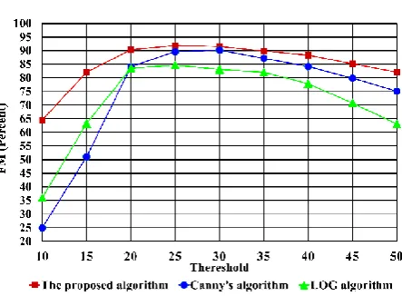
Measure is the harmonic average of Precision and Recall. F-Measure diagram (Figure 9) shows higher values of the proposed algorithm in all the thresholds.

Rosin-Venkatesh [22] is multiplication of True Positive rate (Recall) and True Negative rate. Rosin-Venkatesh diagram (Figure 10) shows higher values of the proposed algorithm in all the thresholds.

Fig 8: ROC diagram for comparison to Canny’s algorithm and LOG algorithm having similar parameters

Fig 9: F-Measure diagram for comparison to Canny’s algorithm and LOG algorithm having similar parameters

Fig 10: Rosin-Venkatesh diagram for comparison to Canny’s algorithm and LOG algorithm having similar

parameters

3.2

Evaluation of locality

There are three reasons that illustrate why the proposed algorithm does not displace edges.

2. Selecting pixels with gradients that are greater than gradients of their neighborhood, leads to selecting pixels that are located in more intensity changes. So for them, probability of being edge is higher.

3. The proposed algorithm uses small smoothing filter that keeps displacements low.

Fig 11: Applied image for evaluation of locality

For evaluation of locality of edges, a separate evaluating program was implemented in C# and one of the famous images in edge detection field was used. Figure 11 illustrates this image that contains types of straight, diagonal and curve lines. So this is appropriate for evaluation of locality.

Fig 12: Evaluated area of the outputs with similar parameters compared to the white area in the main image.

Results of: a) The proposed algorithm with average filter, b) The proposed algorithm with Gaussian filter, c)

Canny’s algorithm

Figure 12 shows the output of edge detectors. The area of white pixels in Figure 11 must be close to the area of shaded pixels in Figure 12. Whatever this area is closer to the area of white pixels in the main image (Figure 11), edge detector keeps locality better. Moreover, calculating the area of objects in images is one of the goals of edge detection.

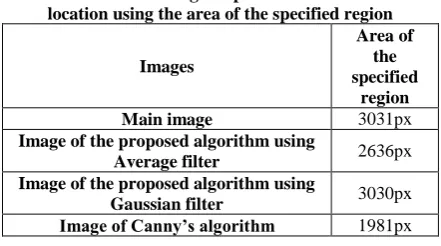
Shaded area in Figure 12 and white area in Figure 11 were calculated by evaluating program. For determining influence of Average and Gaussian filters on the measure of displacements, the proposed algorithm was implemented with each of these filters, and the results were evaluated. Results of this evaluation are presented in Table 1.

Results in Table1 show that the shaded area in output of the proposed algorithm is close to the white area in the main image while there is larger difference for shaded area of the output of Canny’s algorithm. Thus Canny’s algorithm makes edges closer together.

This difference for the proposed algorithm is 395 pixels while this difference for Canny’s algorithm is 1050 pixels. Also the difference for the proposed algorithm with Gaussian filter is one pixel. Thus, Gaussian filter is more precise in locality than the Average filter. According to these results, Gaussian filter and Average filter are both acceptable for the proposed algorithm, but the Average filter is a bit faster.

Table 1. Evaluation of edge displacements from its correct location using the area of the specified region

Images

Area of the specified

region

Main image 3031px

Image of the proposed algorithm using

Average filter 2636px

Image of the proposed algorithm using

Gaussian filter 3030px

Image of Canny’s algorithm 1981px

Therefore we can conclude that in this algorithm, there are fewer displacements of edges compared to Canny’s algorithm.

3.3

Evaluation of execution time

There are different reasons for higher speed of the proposed algorithm compared to speed of Canny’s algorithm.

1. Removing many pixels using average of their neighborhood values and not calculating them in the following steps.

2. Early comparing of threshold against late comparing of threshold in Canny’s algorithm. This leads to removing many other pixels from the following calculations. 3. Not calculating the angle of each pixel based on tangent.

Obtaining angle class directly for pixels which are candidate for being edge until that step.

4. Running Non-Maximum suppression only on pixels which are candidate for being edge until that step. 5. In Non-Maximum suppression of Canny’s algorithm,

the number of comparisons for each pixel is two, while that is one in the proposed algorithm.

6. In the proposed algorithm, there is computational overlapping for calculating rows and columns in thresholding, and also for calculating gradient and average of neighborhood.

For evaluation of execution time, this algorithm should be compared to Canny’s algorithm which is high quality algorithm much like the proposed algorithm.

For this purpose, Method of the proposed algorithm and Canny’s algorithm were put in “For loop” with 100 repetitions in each threshold and average of execution time was extracted. Lenna image and the computer with 2.8 GHz CPU and 3G RAM were used for this test.

As Table 2 shows, because Canny’s algorithm checks threshold at the end of the algorithm, changing thresholds does not change the execution time. The subject that affects the speed of Canny’s algorithm is to trace pixels between two thresholds in order to find a path to the edges.

Table 2. Comparison of the execution time of two algorithms using 512*512 Lenna image

Algorithm Threshold

Time of the Proposed algorithm (Second)

Time of Canny’s algorithm

(Second)

10 0.1560002 0.2184003

20 0.1404002 0.2028004

30 0.1404002 0.2028004

The proposed algorithm, in thinning and reduction of noise steps, only works on pixels which are darker or equal to average of their neighborhood and subtraction of their neighboring pixels is greater than threshold as well. Upper thresholds remove more pixels from the following calculations. That is why the value of threshold is efficient for execution time. Whatever a threshold is higher, speed is also higher. A more important result is that the speed of the proposed algorithm is higher in all thresholds. Figure 13 shows the comparison of execution time in both algorithms.

3.4

Visual evaluation of the proposed

algorithm results

Visual evaluation is not easy and needs more attention. Figures 14-17 illustrate comparison of the proposed algorithm to Canny’s algorithm. Figure14 shows that the continuity on the back wing, left wing and right wing for output of the proposed algorithm (Figure 14.b) is better than the output of Canny’s algorithm.

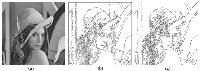
Also Figure 15 shows the difference of quality in two algorithms. Both images are outputs with similar parameters. Lenna’s eyelashes in the output of the proposed algorithm are clear while they are somehow distorted in the output of Canny’s algorithm. Similar cases are found in Figure 16. Also Figure 17.b shows more details on the windows of building.

4.

CONCLUSIONS

Execution time and quality are two challenges for edge detectors. The proposed algorithm achieved good quality in lower time. In many researches, only some aspects of edge detectors evaluation are investigated and some of the researches only concentrate on visual evaluation which is not so precise. This research investigated more aspects of the edge detectors evaluation.

This research tried to overcome some practical limitations of gradient based algorithms. As the diagrams illustrated, statistical evaluation of the output pixels confirmed a considerable accuracy of the proposed algorithm results. Visual evaluation also confirmed statistical evaluation results. Evaluation of locality of edges indicated that displacements of edges in the proposed algorithm are low. Execution time diagram illustrated that the speed of this algorithm is higher than the speed of Canny’s high quality algorithm. Thus this algorithm can be used for real-time programs.

Fig 13: Comparison of the execution times of two algorithms having similar parameters using Lenna image

Fig 14: Visual comparison of the output results of two algorithmshaving similar parameters. a) Result of the

proposed algorithm, b) Result of Canny’s algorithm

Fig 16: Visual comparison of the output results of two algorithms having similar parameters. b) Result of the proposed algorithm, c) Result of Canny’s algorithm

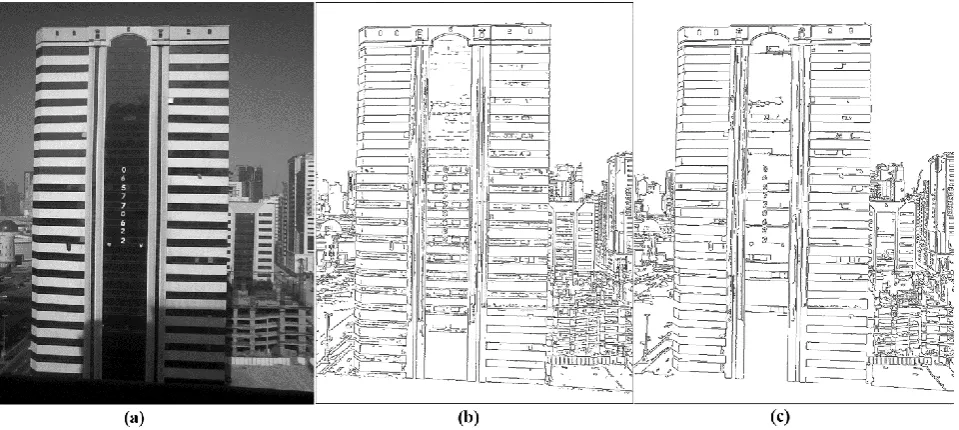
Fig 17: Visual comparison of the output results of two algorithms having similar parameters. b) Result of the proposed algorithm, c) Result of Canny’s algorithm

5.

REFERENCES

[1] Enayatifar, R., Meybodi, M. R. 2009. Adaptive Edge Detection via Image Statistic Features and Hybrid Model of Fuzzy Cellular Automata and Cellular Learning Automata. Proceedings of 2009 International Conference on Information and Multimedia Technology (ICIMT). IEEE Computer Society, Jeju Island, South Korea. 273-278.

[2] Patel, D.K., More S.A. 2013. Edge Detection Technique by Fuzzy Logic and Cellular Learning Automata using Fuzzy Image Processing. International Conference on Computer Communication and Informatics (ICCCI). 1 - 6.

[3] Sato, S., Kanoh, H. 2010. Evolutionary Design of Edge Detector Using Rule Changing Cellular Automata. Second World Congress on Nature and Biologically Inspired Computing, in Kitakyushu, Fukuoka, Japan. 15-17.

[4] Priego, B., Bellas, F., Souto, D., López-Peña, F., Duro, R.J. 2012. Evolving Cellular Automata for Detecting Edges in Hyperspectral Images. IEEE World Congress

on Computational Intelligence June, Brisbane, Australia. 1-6.

[5] Qu, G. 2001. Directional Morphological Gradient Edge Detector. PHD Thesis, Santa Clara University.

[6] Li, T., G., Wang, S.P., Zhao, N. 2009. Gray-scale edge detection for gastric tumor pathologic cell images by morphological analysis. Computers in Biology and Medicine. 39(11), 947—952.

[7] Li, J. 2003. A wavelet approach to edge detection. Sam Houston State University.

[8] Wenchang, S., Song, J., Lin Z. 2009. Wavelet Multi-scale Edge Detection Using Adaptive threshold. IEEE.1-4.

[9] Guo, F., Yang, Y., Chen, B., Guo, L. 2010. A novel multi-scale edge detection technique based on wavelet analysis with application in multiphase flows. Powder Technology. 202 (1-3), 171–177.

[11]Lopez-Molinaa, C., De Baets, B., C., Bustince, H. 2011. Generating fuzzy edge images from gradient magnitudes. Computer Vision and Image Understanding. 115(11), 1571–1580.

[12]Oram, J.J., McWilliams, J.C., Stolzenbach, K.D. 2008. Gradient-based edge detection and feature classification of sea-surface images of the Southern California Bight, Remote Sensing of Environment. 112 (5), 2397–2415. [13]Yu, J., Wang, Y., Shen, Y. 2008. Noise reduction and

edge detection via kernel anisotropic diffusion. Pattern Recognition Letters. 29 (10), 1496–1503.

[14]Canny, J. 1983. Finding edges and lines in image. M. S. thesis. MIT.

[15]Xiao W., Hui X. 2010. An Improved Canny Edge Detection Algorithm Based on Predisposal Method for Image Corrupted by Gaussian Noise. IEEE World Automation Congr. 113–116.

[16]Biswas, R., Sil, J. 2012. An Improved Canny Edge Detection Algorithm Based on Type-2 Fuzzy Sets. Procedia Technology. 4, 820 – 824.

[17] Xue, L.Y., Pan, J.J. 2009. Edge detection combining wavelet transform and Canny operator based on fusion rules. IEEE Proceedings of the 2009 international conference on wavelet analysis and pattern recognition. 324-328.

[18] Kim, D.S., Lee W.H., Kweon, I.S. 2004. Automatic edge detection using 3 • 3 ideal binary pixel patterns and fuzzy-based edge thresholding. Pattern Recognition Letters. 25 (1), 101–106.

[19] "Boundary Detection Benchmark: Image Ranking"

[Online]. Available:

http://www.eecs.berkeley.edu/Research/Projects/CS/visi on/bsds/bench/html/images.html.

[20] Lopez-Molinaa, C., De Baets, B., C., Bustince, H. 2013. Quantitative error measures for edge detection, Pattern Recognition. 46(4), 1125–1139.

[21] Fawcett, T. 2006. An introduction to ROC analysis. Pattern Recognition Letters. 27(8), 861–874.