A comparative analysis of correlation skew modeling techniques for CDO index tranches

Munich Personal RePEc Archive

A comparative analysis of correlation

skew modeling techniques for CDO index

tranches

Claudio, Ferrarese

King’s College London

8 September 2006

Online at

https://mpra.ub.uni-muenchen.de/1668/

A Comparative Analysis of Correlation

Skew Modeling Techniques for CDO

Index Tranches

by

Claudio Ferrarese

Department of Mathematics

King’s College London

The Strand, London WC2R 2LS

United Kingdom

Email: [email protected]

Tel: +44 799 0620459

8 September 2006

Abstract

In this work we present an analysis of CDO pricing models with a focus on “correlation skew models”. These models are extensions of the classic sin-gle factor Gaussian copula and may generate a skew. We consider examples with fat tailed distributions, stochastic and local correlation which generally provide a closer fit to market quotes. We present an additional variation of the stochastic correlation framework using normal inverse Gaussian distri-butions. The numerical analysis is carried out using a large homogeneous portfolio approximation.

Contents

1 Introduction 2

2 CDOs pricing 4

2.1 CDO tranches and indices: iTraxx, CDX . . . 4

2.2 Pricing Models overview . . . 8

2.2.1 Copulas . . . 10

2.2.2 Factor models . . . 12

2.2.3 Homogeneous portfolios and large homogeneous port-folios . . . 14

2.2.4 Algorithms and fast Fourier transform for CDOs pricing 16 3 Correlation skew 19 3.1 What is the correlation skew? . . . 19

3.2 Analogy with the options market and explanation of the skew 21 3.3 Limitations of implied correlation and base correlation . . . . 22

4 Gaussian copula extensions: correlation skew models 25 4.1 Factor models using alternative distributions . . . 25

4.1.1 Normal inverse Gaussian distributions (NIG) . . . 27

4.1.2 α-stable distributions . . . 30

4.2 Stochastic correlation . . . 32

4.3 Local correlation . . . 37

4.3.1 Random factor loadings . . . 37

4.4 Stochastic correlation using normal inverse Gaussian . . . 40

5 Numerical results 44 5.1 Pricing iTraxx with different models . . . 44

Chapter 1

Introduction

The credit derivatives market has grown quickly during the past ten years, reaching more than US$ 17 trillion notional value of contracts outstanding in 2006 (with a 105% growth during the last year) according to International Swaps and Derivatives Association (ISDA)1_{. The rapid development has}

brought market liquidity and improved the standardisation within the mar-ket. This market has evolved with collateralised debt obligation (CDOs) and recently, the synthetic CDOs market has seen the development of tranched index trades. CDOs have been typically priced under reduced form models, through the use of copula functions. The model generally regarded as a mar-ket standard, or the “Black-Scholes formula” for CDOs, is considered to be the Gaussian copula (as in the famous paper by Li [36]). Along with market growth, we have seen the evolution of pricing models and techniques used by practitioners and academics, to price structured credit derivatives. A general introduction on CDOs and pricing models is given in_§2. In _§3.1 we describe and attempt to explain the existence of the so called “correlation skew”. An-other standard market practice considered here is the base correlation. The core part of this work concentrates on the analysis of the extensions of the base model (i.e. single factor Gaussian copula under the large homogeneous portfolio approximation). These extensions have been proposed during the last few years and attempt to solve the correlation skew problem and thus produce a good fit for the market quotes. Amongst these model extensions, in_§4 we use fat-tailed distributions (e.g. normal inverse Gaussian (NIG) and

α-stable distributions), stochastic correlation and local correlation models to price the DJ iTraxx index. In addition to these approaches, we propose the “stochastic correlation NIG”, which represents a new variation of the stochastic correlation model. In particular we use the normal inverse

Gaus-1

Chapter 2

CDOs pricing

In this chapter, after a quick introduction to CDOs and the standardised tranche indices actively traded in the market, we present the most famous approaches, such as copula functions and factor models, used to price struc-tured credit derivatives.

2.1

CDO tranches and indices: iTraxx, CDX

CDOs allow, through a securitisation technique, the repackaging of a port-folio credit risk into tranches with varying seniority. During the life of the transaction the resulting losses affect first the so called “equity” piece and then, after the equity tranche as been exhausted, the mezzanine tranches. Further losses, due to credit events on a large number of reference entities, are supported by senior and super senior tranches. The difference between a cash and synthetic CDO relies on the underlying portfolios. While in the former we securitise a portfolio of bonds, asset-backed securities or loans, in the latter kind of deals the exposition is obtained synthetically, i.e. through credit default swaps (CDS) or other credit derivatives. The possibility of spread arbitrage1_{, financial institutions’ need to transfer credit risk to free}

up regulatory capital (according to Basel II capital requirements), and the opportunity to invest in portfolio risk tranches have boosted the market. In particular it has been very appealing for a wide range of investors who, hav-ing different risk-return profiles2_{, can invest in a specific part of CDO capital}

1

An common arbitrage opportunity exists when the total amount of credit protection premiums received on a portfolio of, e.g., CDS is higher than the premiums required by the CDO tranches investors.

2

structure. Clearly, CDO investors are exposed to a so called “default correla-tion risk” or more precisely to the co-dependence of the underlying reference entities’ defaults3_{. This exposure varies amongst the different parts of the}

capital structure: e.g. while an equity investor would benefit from a higher correlation, the loss probability on the first loss piece being lower if correla-tion increases, a senior investor will be penalised if the correlacorrela-tion grows, as the probability of having extreme co-movements will be higher.

CDO tranches are defined using the definition of attachmentKA and

de-tachment pointsKDas, respectively, the lower and upper bound of a tranche.

They are generally expressed as a percentage of the portfolio and determine the tranche size. The credit enhancement of each tranche is then given by the attachment point. For convenience we define the following variables:

• n- the number of reference entities included in the collateral portfolio (i.e. number of CDS in a synthetic CDO);

• Ai- the nominal amount for the i−th reference entity;

• δi- the recovery rate for thei−th reference entity;

• T- the maturity;

• N- the number of periods or payment dates (typically the number of quarters);

• B(0, t)- the price of a risk free discount bond maturing at t;

• τi- the default time for the i−th reference entity;

• sBE- the break-even premium in basis point per period (i.e. spread).

The aggregate loss at time t is given by:

L(t) =

n X

i=1

Ai(1−δi)1{τi≤t}, (2.1)

assuming a fixed recovery rate δ, notional equal to 1 and the same exposure to each reference entity in the portfolio Ai =A= _N1, the loss can be written

3

as follows:

L(t) = 1

N(1−δ)

n X

i=1

1_{τi≤t}, (2.2)

For every tranche, given the total portfolio loss in 2.2, the cumulative tranche loss is given by:

L[KA,KD](t) = max{min[L(t), KD]−KA,0}. (2.3) The so called “protection leg”, which covers the losses affecting the spe-cific tranche and is paid out to the protection buyer, given the following payment dates

0 =t0 < t1 < . . . < tN₋1 < tN =T

can be calculated taking the expectation with respect to the risk neutral probability measure:

ProtLeg[KA,KD]=E

" _N

X

j=1

L[KA,KD](tj)−L[KA,KD](tj−1)

B(t0, tj) #

, (2.4) Similarly, assuming a continuous time payment, the protection leg can be written as follows:

ProtLeg[KA,KD] =E

Z T

t0

B(t0, s)dL[KA,KD](s)

. (2.5)

On the other hand, the so called “premium leg” is generally paid quarterly in arrears4 _{to the protection seller and can be expressed as follows:}

PremLeg[KA,KD]=E

" _N

X

j=1

sBE×∆tj(min{max[KD−L(tj),0], KD−KA})B(t0, tj) #

.

(2.6)

The fairsBE can be easily calculated by:

sBE=

E

h

RT

t0 B(t0, s)dL[KA,KD](s)

i

EhPNj=1∆tj(min{max[KD−L(tj),0], KD−KA})B(t0, tj)

i.

4

In order to price a CDO it is then central to calculate the cumulative portfolio loss distribution necessary to evaluate the protection and premium legs. In the sequel, the loss distribution will be analysed comparing some of the most popular approaches proposed by academics and practitioners, having as a primary goal the fitting of the prices quoted by the market.

Traded indices

As already mentioned, one of the most effective innovations in this market has been the growth of standardised and now liquid index tranches such as DJ iTraxx and DJ CDX. These indices allow investors to long/short single tranches, bet on their view on correlation, hedge correlation risk in a book of credit risks and infer information from the market, computing the correlation implied by the quotes.

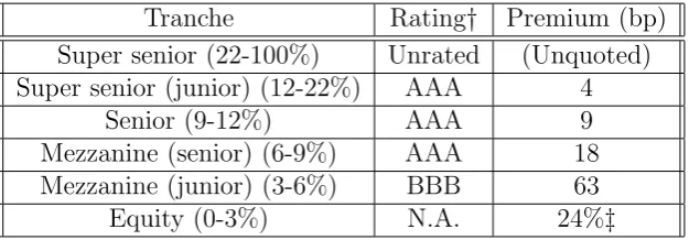
Tranche Rating† Premium (bp) Super senior (22-100%) Unrated (Unquoted) Super senior (junior) (12-22%) AAA 4

Senior (9-12%) AAA 9

Mezzanine (senior) (6-9%) AAA 18 Mezzanine (junior) (3-6%) BBB 63

Equity (0-3%) N.A. 24%_‡

Figure 2.1: DJ iTraxx standard capital structure and prices in basis pints (bp) at 13 April 2006.

Source: CDO-CDS Update: Nomura Fixed Income Research, 4/24/2006.

†These are not official ratings, but only an assessment of the creditworthiness of iTraxx index tranches provided by Fitch, for further information see http://www.fitchcdx.com.

‡ For the equity tranche an upfront premium plus 500 bp running spread is usually quoted.

These indices are build according to the following rules5_:

• they are composed of 125 European (US for the DJ CDX IG) equally weighted investment grade firms;

• transparent trading mechanics and standard maturities;

5

• standardised credit events definitions and ISDA based documentation;

• cross sector index including entities from auto, consumer, energy, in-dustrial, TMT and financial sectors;

• the most liquid entities with the highest CDS trading volume, as mea-sured over the previous 6 months, are chosen for the index composition;

• the index composition is periodically revisited, every new series shares the majority of its names with the previous series.

2.2

Pricing Models overview

In credit models two main approaches have been used:

• Structural models, based on option theory, were introduced by Merton [41] and further developed by e.g. Black and Cox [11], Leland and Toft [35]. Under this approach a default occurs when the value of the firm’s assets drops below the face value of the debt (i.e. strike price), thus considering the stock being a call option on the company’s value.

• Reduced form approach attempts to model the time of the default itself through the use of an exogenously given intensity process (i.e. jump process), see e.g. Jarrow and Turnbull [32], Lando[34], Duffie [19], Hughston and Turnbull [28]. Within the reduced form models, the

incomplete information approach , see Brodyet al. [13] focuses on the modelling of the information available in the market.

In this work we use the intensity based approach. We briefly introduce the main assumptions on which the following is based. Given a standard fil-tered probability space (Ω,_F,P,_{Ft)}, we assume the existence of a pricing

In general, pricing a CDO requires us to model both the risk neutral default probabilities for each name in the portfolio and the joint default dis-tribution of defaults. The risk neutral default probabilities can be calculated following the popular practice of bootstrapping from CDS premiums. Here we summarise the main steps. For a complete exposition we refer to, e.g., Bluhm et al.[12], Li [36, 37], Sch¨onbucher[49] or Lando [34]. Given the stan-dard probability space defined above, we consider the {Ft)-stopping time τi

to model the default of the i₋th obligor in a portfolio, the default proba-bility distribution is given by Fi(t) = P{τi < t} and the probability density

distribution is fi(t). We define the “hazard rate” or “intensity” as follows:

λi(t) =

fi(t)

1₋Fi(t)

. (2.7)

From 2.7 the following O.D.E. can be obtained:

λi(t) = −

dln(1−Fi(t))

dt , (2.8)

and, solving the O.D.E., an expression for the default probability distribution follows:

Fi(t) = 1−e−

❘t

0λi(s)ds_{. (2.9)}

We make a further step defining τi as the first jump of an inhomogeneous

Poisson6 _{process N(t) with parameter Λ(T)−Λ(t) =} RT

t λi(s)ds, then:

P{NT −Nt=k} =

1

k!

Z T

t

λi(s)ds

k

e−❘tTλi(s)ds_{. (2.10)}

In fact, using the fact that _P{Nt = 0}=e−

❘T

t λi(s)ds, the survival probability

for the i₋th obligor can be written, similarly to 2.9, as follows: 1−Fi(t) = e−

❘T

t λi(s)ds. (2.11)

Once the hazard rate7 _λ

i(t) has been defined, it is straightforward to

boot-strap the default probabilities, e.g. a standard practice is to use a piecewise constant hazard rate curve and fit it with the CDS quotes.

In the sequel we assume that risk neutral default probabilities have been calculated for all names in the underlying reference portfolio.

6

In addition an inhomogeneous Poisson process with λi(t) > 0 is characterised by

independent increments andN0= 0. 7

2.2.1

Copulas

Copulas are a particularly useful class of function, since they provide a flexible way to study multivariate distributions. Li [36] was certainly amongst the first to introduce these functions in credit derivatives modelling because of the copulas’ characteristic of linking the univariate marginal distributions to a full multivariate distribution. We present here the definition and an important result regarding copulas. For a full presentation of the argument please refer to e.g. Cherubini et al. [18].

Definition 1 (Copula) A n-dimensional copula is a joint cdf C : [0,1]n

→

[0,1] of a vector u of uniform U(0,1) random variables:

C(u1, u2, . . . , un) =P(U1 < u1, U2 < u2, . . . , Un < un), (2.12)

where ui ∈[0,1], i= 1,2, . . . , n.

Theorem 1 (Sklar theorem) Given H(x1, x2, . . . , xn) the joint

distribu-tion funcdistribu-tion with marginals FX1(x1), FX2(x2), . . . , FXn(xn), then there exists a copula C(u1, u2, . . . , un) such that:

H(x1, x2, . . . , xn) = C(fX1(x1), fX2(x2), . . . , fXn(xn)). (2.13) Furthermore the copula C is given by:

C(u1, u2, . . . , un) =H(F₁−1(u1), F2−1(u2), . . . , Fn−1(un)). (2.14)

In particular, if the Fi, i= 1,2, . . . , n, are continuous, then C is unique.

One of the most used copulas in financial applications is certainly the stan-dard Gaussian copula. We give here the definition and describe how it can be used to model joint default distributions.

Definition 2 (Standard Gaussian copula) The standard Gaussian cop-ula function is given by :

C_ΣG(u1, u2, . . . , un) = ΦΣn(Φ−

1_(u

1),Φ−1(u2), . . . ,Φ−1(un)), (2.15)

where ΦΣ

n is a n variate Gaussian joint distribution function, Σ is a

Using the arguments in §2.2, for the i₋th, i = 1,2, . . . , n name in the portfolio, a default threshold8 _{can be found:}

P{1₋Fi(t) = e−

❘T

t λi(s)ds_{}< U}

i. (2.16)

Ui being a uniform U(0,1) random variable9.

It is then possible to build a joint default time distribution from the marginal distributions Fi(t) =P{τi < t} as follows:

P{τ1 ≤t, τ2 ≤t, . . . , τn ≤t}=CΣG(F1(t), F2(t), . . . , Fn(t))

= ΦΣ_n Φ−1(F1(t)),Φ−1(F2(t)), . . . ,Φ−1(Fn(t))

. (2.18) Using the results in 2.16 and 2.18, a Monte Carlo simulation algorithm can be used to find the joint default time distribution:

• sample a vector z of correlated Gaussian random variables with corre-lation matrix Σ10_;

• generate a vector of uniform random variable u= Φ(z);

• for everyi= 1,2, . . . , nand timet, we have a default if τi =Fi−1(ui)<

t;

• evaluate the joint default distribution;

• repeat these steps for the required number of simulations.

Credit derivatives can now be priced since the cumulative portfolio loss distribution follows from the joint default distribution calculated according to the previous algorithm.

8

Note that this approach is based on the simple idea of a default event modelled by a company process falling below a certain barrier as stated in the original Merton structural model [41]

9

Using that F(t) is a distribution function then

P{F(t)< t_}=P{F−1

(F(t))< F−1

(t)_}=P{t < F−1

(t)_}=F(F−1

(t)) =t

(2.17)

it follows that F(t) is a uniformU(0,1) random variable and so is 1−F(t).

10

Given a vectorv_{of independent Gaussian random variables and using an appropriate}

decomposition, e.g. Cholesky, of Σ = CCT_{, a vector of correlated Gaussian random}

A number of alternative copulas such as, e.g. Student t, Archimedean, Marshall-Olkin copulas have been widely studied and applied to credit deriva-tives pricing with various results, see e.g. Galiani [24], Sch¨onbucher[47, 49], Chaplin [17] for a complete description.

We conclude this section recalling that the algorithm described above can be particularly slow when applied to basket credit derivatives11_pricing,

hedg-ing or calibration. In the followhedg-ing sections we describe another approach to overcome the main limitations described above.

2.2.2

Factor models

In this section we present a general framework for factor models. The idea behind factor models is to assume that all the names are influenced by the same sources of uncertainty. For simplicity we will use a so called single factor model, i.e. there is only one common variable influencing the dynamics of the security, the other influences are idiosyncratic. Factor models have widely been applied by many authors12_{to credit derivatives modelling for essentially}

two reasons:

• factor models represent an intuitive framework and allow fast calcula-tion of the loss distribucalcula-tion funccalcula-tion without the need to use a Monte Carlo simulation;

• there is no need to model the full correlation matrix, which represents a challenging issue, since default correlation is very difficult to estimate, i.e. joint defaults are particulary uncommon and there is generally a lack of data for a reliable statistic, and CDS spread correlation or equity correlation13 _{can only be assumed as a proxy of default correlation,}

these quantities being influenced by other forces, e.g. liquidity.

Factor models can then be used to describe the dependency structure amongst credits using a so called “credit-vs-common factors” analysis rather than a pairwise analysis.

An example of factor model is given by the following expression:

Vi =√ρY + p

1₋ρǫi, (2.19)

11

Synthetic CDOs or indices have generally more than 100 reference entities and defaults are “rare events” especially when the portfolio is composed of investment grade obligors. A large number of simulation is then needed for reliable results.

12

See e.g. Laurent and Gregory [?_{], Andersen} et al. [3], Finger [22], Hull and White [30], Sch¨onbucher [46] or Galianiet al. [25].

13

Moreover the analysis is complicated by the fact that, given e.g. the index iTraxx Europe, it is necessary to estimateN(N₋1)1

whereVi is a individual risk process andY, ǫi, i= 1,2, . . . , nare i.i.d. Φ(0,1).

We note that, conditioning on the systemic factor Y, the Vi are pairwise

independent. Moreover, the random variables Y and ǫi being independent,

it follows that Vi is Φ(0,1). It is then possible to calculate the correlation

between each pair as follows:

Corr [Vi, Vj] = E[Vi, Vj] =E[√ρY + p

(1−ρ)ǫi,√ρY + p

(1−ρ)ǫj]

= ρ_E[Y2] =ρ.

For each individual obligor we can calculate the probability of a default happening before maturity t, P{τi ≤t}, as the probability that the value of

the company Vi falls below a certain threshold ki:

P{Vi ≤ki} = P

n√

ρY +p1₋ρǫi ≤ki o

= P

ǫi ≤

ki−√ρY

√

1₋ρ

= Φ

_k

i−√ρY

√

1₋ρ

.

The value of the barrier ki can be easily calculated following the theory

presented in§2.2. Assuming that the time of defaultτi is the time of the first

jump of an inhomogeneous Poisson processN(t) and using the survival prob-ability found in the equation 2.11, the probprob-ability of default for a single name is then given by P{τi ≤ t} = 1−e

❘t

0λi(s)ds _{= F}

i(t) = P{Vi ≤ ki} = Φ(ki).

The value of the barrier14 _{can then be written as follows: k}

i = Φ−1(Fi(t)).

Using the tower property of conditional expectation we can calculate the probability of default with the following expression:

P{Vi ≤ki} = E[1_{Vi≤ki}] =E

E1_{Vi≤ki}|Y =y

= E

P

ǫi ≤

ki−√ρy

√

1₋ρ

Y =y

= E

Φ

_k

i−√ρy

√

1₋ρ

= Z ∞ −∞ Φ _k

i−√ρy

√

1₋ρ

dFY(y). (2.20)

14

Furthermore, using that, conditioning onY the defaults of the underlyings are independent, the loss distribution for a sequence of names is given by:

P{τ1 ≤t, τ2 ≤t, . . . , τn≤t} = E[E[1{τ1≤t,τ2≤t,...,τn≤t}|Y =y]]

= E[E[1_{τ1≤t}|Y =y]E[1{τ2≤t}|Y =y]. . .E[1{τn≤t}|Y =y]]

= Eh

n Y

i=1

pi(t|Y) i = Z ∞ −∞ n Y i=1

pi(t|y)dFY(y). (2.21)

where pi(t|y) = Φ

h_k

i−√ρy

√

1−ρ i

.

The expression in 2.21, similarly to the definitions presented in _§2.2.1 represents the so called “one-factor Gaussian copula”:

C_ρG =

Z ∞

−∞

n Y

i=1

pi(t|y)dFY(y). (2.22)

2.2.3

Homogeneous portfolios and large homogeneous

portfolios

The framework described in the previous sections can be easily used to price CDOs making further assumptions on the nature of the underlying obligors. We consider here two main approximations: homogeneous portfolios(HP), i.e. the portfolio consists of identical obligors, and large homogeneous port-folios(LHP), under which the number of obligors is very largen_→∞. Under the homogeneous portfolios approximation we use same recovery rate15 _δ

and default probability p for every name, the loss given default would also be identical for all the entities in the portfolio. Using the conditional de-fault probability pi(t|y) = Φ

h_k

i−√ρy

√

1−ρ i

and the fact that, conditional upon the common factor Y the defaults in the portfolio are independent events, it is possible to write the following formula for P{L=i(1₋δ)_}:

P{L=i(1₋δ)_} =

Z ∞ −∞ n i

p(t_|y)i₍₁

−p(t_|y))n−i_dF

Y(y). (2.23)

15

where the number of defaults (conditioning on Y) follows a binomial distri-bution _BIN(n, p(t_|y)).

The equation 2.23 can be easily solved numerically using e.g. Simpson’s rule or another numerical integration technique. An expression for the dis-tribution of the aggregate loss GL is then given by:

GL(i(1−δ)) =P{L≤i(1−δ) = i X

m=0

P{L=m(1₋δ)_} (2.24) The large homogeneous portfolios approximation allows us to express the loss distribution function in a closed form, given that for a large portfolio the latent variable has a strong influence. This result, firstly proved by Vasicek [52], states that as n _{−→ ∞}, by the law of large numbers, the fraction of defaulted credits in the portfolio converges to the individual default proba-bility:

P

L

n −p(t|y)

> ε

Y =y

→0, (2.25)

∀ε >0 and n_→∞.

Assuming for simplicity zero recoveries and that L, conditioning on Y, follows a Binomial distribution, we can immediately write down the mean and variance as follows:

E[L_|Y =y] =np(t_|y), and

Var[L_|Y =y] =np(t_|y)(1₋p(t_|y)). It is then possible to calculate:

ELn|Y =y

=p(t_|y), and

Var_L

n|Y =y

= _n1p(t_|y)(1−p(t_|y)). Since, as n_→∞, Var_L

n|Y =y

→0, given Y =y, it follows that

L

Using this result, i.e. L

n(1−δ) −→ p(t|y), given any x ∈ [0,1], an expression

for the loss distribution function G(x) can be calculated as follows:

G(x) = P{pi(t|Y)≤x}

= P

Φ

_k

i−√ρY

√

1₋ρ

≤x

= P

_k

i −√ρY

√

1₋ρ ≤Φ −1_(x)

= P

Y > ki−

√

1₋ρΦ−1_(x)

√_ρ

= 1₋P

Y _≤ ki−

√

1₋ρΦ−1_(x)

√_ρ

= Φ

√

1₋ρΦ−1_(x)−k

i

√_ρ

(2.26)

2.2.4

Algorithms and fast Fourier transform for CDOs

pricing

We conclude this chapter with a quick overview of two amongst the most popular techniques used to price CDOs when the idealised LHP or HP as-sumptions don’t hold, i.e. the underlying obligors have different default probabilities and they are a finite number. For simplicity we will continue to assume the same weight for each underlying name in the portfolio (which is generally not a problem for index tranches) and the same recovery rates. We will focus on the Hull and White stile algorithm, see [30] and on the fast Fourier transform, see e.g. Laurent and Gregory [27] or Sch¨onbucher [48] to solve the problem. The first method is based on a recursive approach and uses that, conditioning on Y = y, the default events are independent. We present here a popular version of this algorithm.

Denoting with P(n)_{(i) the probability}16 _{of having i defaults from the n}

names, and with pi the default probability of the i−th company, we can

write:

P(1)(i) =

1₋p1 for i= 0,

p1 for i= 1. 16

P(2)(i) =

 



(1₋p1)(1−p2) for i= 0,

p1(1−p2) +p2(1−p1) for i= 1,

p1p2 for i= 2.

Observing thatP(2)(i) can be written recursively:

P(2)(i) = P(1)(i)(1₋p2) +P(1)(i−1)p2,

and for 2< j < n,

P(j+1)(i) =P(j)(i)(1₋pj+1) +P(j)(i−1)pj+1.

Using the recursion it is then possible to find an expression for the con-ditional portfolio loss P(n)(i_|y).

Analogously to the method described with formula 2.23, integrating out the latent variable Y we can recover the expression for the (unconditional) portfolio loss:

P{L=i(1−δ)} =

Z ∞

−∞

P(n)(i|y)dFY(y). (2.27)

We consider here a second approach to solve this problem with the fast Fourier transform(FFT). This approach shares with the previous one the conditional independence assumption, i.e. conditional on the latent variable

Y, the defaults of the obligors are independent random variables. Given this assumption and the individual loss given default (1−δi) = li for every

name in the pool, the portfolio loss can be written as a sum of independent random variable: Z = Pn_i=1li. The characteristic function, conditional on

the common factor Y, is then given by: EeiuZ|Y = _EneiuPni=1li_|Y

o

= _E

eiu(li)_|Y

Eeiul2_{|Y . . .}

Eeiuln_{|Y . (2.28)}

The characteristic function for thei₋th obligor can be written as: Eeiuli|Y _{= e}iuli_p

i(t|y) + (1−pi(t|y))

= 1 + [eiuli _−1]p

Inserting the characteristic function 2.29 into the 2.28 we can express the portfolio characteristic function (conditional on Y) as follows:

EeiuZ|Y =

n Y

i=1

1 + [eiuli _−1]p

i(t|y)

, (2.30)

and integrating out the common factor we get the unconditional charac-teristic function:

ˆ

h(u) =_E

eiuZ =

Z ∞

−∞

n Y

i=1

1 + [eiuli _−1]p

i(t|y)

dFY(y). (2.31)

The integral in 2.31 can be solved numerically by, e.g., quadrature tech-nique or Monte Carlo simulation. Once we have found the characteristic function of the portfolio loss ˆh(u) the density function can be found using the fast Fourier transform17 _{which is a computationally efficient.}

17

We recall that given the Fourier transform ˆh(u), the density functionh(t) is given by

1 2_π

R∞

Chapter 3

Correlation skew

In this chapter we briefly present some of the main concepts used to imply correlation data from the market quotes. We describe implied correlation and different tranches’ sensitivity to correlation, the correlation smile ob-tained from market data, and we present a standard market practice used by practitioners in correlation modelling: base correlation.

3.1

What is the correlation skew?

Although the single factor copula model, particularly in its Gaussian version presented in _§2, is in general not able to match the market quotes directly, it has become a market standard for index tranches pricing. Amongst the limitations1 _{of this model that can explain its partial failure, there is}

cer-tainly the fact that Gaussian copula has light tails and this has an important impact on the model’s ability to fit market quotes, defaults being rare events. To overcome this restriction it is enough to modify the correlation parameter into the single factor model: other things being equal, increasing the cor-relation parameter leads to an increase of the probability in the tails, thus leading to either very few or a very large number of defaults. The new loss distributions, generated by varying the correlation parameter, are able to fit the market quotes obtaining the so called “implied correlation” or “com-pound correlation”. Implied correlations obtained with this practice can be interpreted as a measure of the markets view on default correlation.

Implied correlation has been widely used to communicate “tranche corre-lation” between traders and investors using the Gaussian copula as a common

1

framework2_{. The possibility to observe market correlation represents a very}

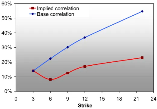
useful resource for dealers who can check the validity of the assumptions used to price bespoken CDOs, non standardised tranches or other exotic structured credit products, with the market quotes for the relevant stan-dardised index. This practice reveals the existence of a “correlation smile” or “correlation skew” which generally takes, as shown in the figure 3.1, the following shape: the mezzanine tranches typically show a lower compound correlation than equity or senior tranches, and for senior and super senior a higher correlation is necessary than for equity tranche.

0% 10% 20% 30% 40% 50% 60%

0 3 6 9 12 15 18 21 24

Strike

Implied correlation Base correlation

Figure 3.1: Implied correlation and base correlation for DJ iTraxx on 13 April 2006. On the X axis we report the detachment point (or strike) for each tranche and on the Y axis the correlation level for both implied correlation or base correlation.

2

3.2

Analogy with the options market and

ex-planation of the skew

The existence of a correlation skew is far from being obvious: since the corre-lation parameter associated with the model does not depend on the specific tranche priced, we would expect an almost flat correlation. The correlation smile can be described through an analogy with the more celebrated volatility smile (or skew): i.e. implied volatility in the Black-Scholes model changes for different strikes of the option. The existence of volatility skew can be explained by two main lines of argument: the first approach is to look at the difference between the asset’s return distribution assumed in the model and the one implicit in the market quotes3_{, while the second is to consider the}

general market supply and demand conditions, e.g. in a market that goes down traders hedge their positions by buying puts.

The correlation smile can be considered in a similar way: we can find explanations based either on the difference between the distribution assumed by the market and the specific model, or based on general market supply and demand factors. Within this analysis, we report three4 _{explanations for the}

correlation smile which, we believe, can explain the phenomena.

• Although the liquidity in the market has grown consistently over the past few years, demand and supply circumstances strongly influence prices. Implied correlations reflect the strong interest by “yield search-ing” investors in selling protection on some tranches. As reported by Bank of England [10]:“the strong demand for mezzanine and senior tranches from continental European and Asian financial institutions may have compressed spreads relative to those of equity tranches to levels unrepresentative of the underlying risks”. To confirm this argu-ment we can add that banks need to sell unrated equity pieces in order to free up regulatory capital under the new Basel II capital requirement rules.

• segmentation among investors across tranches as reported by Amato and Gyntelberg [2]:“different investor groups hold different views about correlations. For instance, the views of sellers of protection on equity tranches (e.g. hedge funds) may differ from sellers of protection on mez-zanine tranches (e.g. banks and securities firms). However, there is no

3

The Black-Scholes model assumes that equity returns are lognormally distributed while the implicit distribution, see e.g Hull [29], has fatter lower tail and lighter upper tail.

4

compelling reason why different investor groups would systematically hold different views about correlations.”

• the standard single-factor gaussian copula is a faulty model for the full capital structure of CDOs index tranches. The reasons may be found in the main assumptions of the model: i.e. the implicit default distribution has fatter tails than the Gaussian copula, recovery rates and default are not independent5_{, and recovery rates are not fixed but}

could be stochastic.

3.3

Limitations of implied correlation and base

correlation

Implied correlation has been a very useful parameter to evince information from the market: e.g. if there is a widening of the underlying index spread and the implied correlation on the equity piece has dropped, the fair spread of an equity tranche would most likely rise. This would be a consequence of the fact that the market is implying an increased idiosyncratic risk on few names which would affect the junior pieces. This would probably not affect the rest of the capital structure.

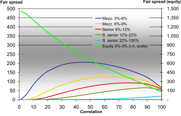
The compound correlation is a useful tool, although it has a few problems that limit its utility: as shown in figure 3.2, mezzanine tranches, not being monotonic in correlation, may not have an implied correlation or they may have multiple implied correlation6 _{(typically two); there are difficulties in}

pricing bespoken tranches consistently with standard ones because of the smile; and there is an instability issue with implied correlation, i.e. a small change in the spread for mezzanine tranches would result in a big movement of the implied correlation, as we can see in figure 3.2.

Because of these limitations, market participants have developed the so called “base correlation”. The concept was introduced by McGinty et al.

[40] and can be defined as the correlation implied by the market on (virtual) equity pieces 0₋KD%. In its original formulation it was extracted using the

large homogeneous pool assumption. A popular7 _{recursion technique can be}

applied to DJ iTraxx as follows:

• the first base correlation 0-3% coincides with the first equity implied correlation;

5

As reported by Altmanet al. [1]:“recovery rates tend to go down just when the number of defaults goes up in economic downturns”.

6

Multiple implied correlation are problematic for hedging.)

7

0 50 100 150 200 250 300 350 400 450 500

0 10 20 30 40 50 60 70 80 90 100

Correlation

-150 300 450 600 750 900 1,050 1,200 1,350 1,500

Fair spread (equity)

Mezz. 3%-6% Mezz. 6%-9% Senior 9%-12% S. senior 12%-22% S. senior 22%-100% Equity 0%-3% (r.h. scale)

Fair spread

Figure 3.2: Correlation sensitivity for DJ iTraxx on 13 April 2006. On the

X axis we report the correlation parameter and on theY axis the fair spread value (expressed in basis points) for each tranche. For the equity tranche a different scale for the fair spread is used, which is reported on the right hand side. From the chart we can see that mezzanine tranches are not monotonic in correlation.

• price the 0-6% tranche combining the 0-3% and the 3-6% tranches with premium equal to the 3-6% tranche’s fair spread and correlation equal to the 0-3% base correlation;

• The 0-6% price is simply the price of the 0-3% tranche with the 3-6% premium, being a 3-6% tranche with the 3-6% premium equal to zero, and can be used to imply the base correlation for the 0-6% tranche, using the standard pricing model;

• using the 0-6% tranche base correlation recursively, we can then find the price of the 0-6% tranche with the 6-9% fair spread;

pre-vious price;

• the procedure has to be iterated for all the tranches.

Base correlation represents a valid solution to the shortcomings of im-plied correlations obtained using the Gaussian copula: especially the prob-lem relating to existence is generally solved (excluding unquoted super senior tranche) and the hedging obtained using base correlation offers better per-formance than the one obtained using implied correlations8_{. However, this}

technique is not solving all the problems related to the correlation skew. Amongst the main limitations of base correlation we recall that the valua-tion of off-market index tranches is not straightforward and depends on the specific interpolative technique of the base correlation.

8

Chapter 4

Gaussian copula extensions:

correlation skew models

The insufficiency of the single factor Gaussian model to match market quotes has already been emphasised by many practitioners and academics and can be summarised as follows:

• relatively low prices for equity and senior tranches;

• high prices for mezzanine tranches.

For a good understanding of the problem it is central to look at the cumulative loss distribution resulting from the Gaussian copula and the one implied by the market, as in figure 4.1: a consistently higher probability is allocated by the market to high default scenarios than the probability mass associated with a Gaussian copula model (which has no particularly fat upper tail). Furthermore, the market assigns a low probability of zero (or few) defaults, while in the Gaussian copula it is certainly higher. In this chapter we look at some of the proposed extensions to the base model and, mixing two of these different approaches, we propose a new variation of correlation skew model.

4.1

Factor models using alternative

distribu-tions

A factor model can be set up using different distributions for the common and specific factors. There is a very rich literature1 _{on copulas that can be}

1

0 10 20 30 40 50 60 70 80 90 100 0.96

0.965 0.97 0.975 0.98 0.985 0.99 0.995 1 1.005

Cumulative loss

Cumulative

p

robability

Gaussian

Market

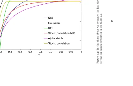
Figure 4.1: In this chart we compare the cumulative portfolio loss using a Gaussian copula and the loss implied by the market. The Y axis reports the cumulative probability, while theX axis reports the cumulative portfolio loss.

used, amongst the most famous we recall the Student t, Archimedean and Marshall-Olkin copulas.

In the sequel two distributions are analysed:

• normal inverse Gaussian;

• α-stable.

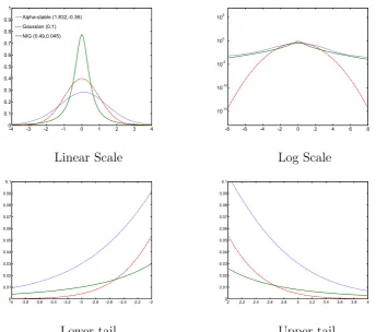
The choice of these two distributions is due to their particular versatility and ability to cope with heavy-tailed processes: appropriately chosen values for their parameters can provide an extensive range of shapes of the distribution. In figure 4.2 these distributions are compared with the Gaussian pdf: the upper and lower tails are higher for both α-stable and NIG, showing that a higher probability is associated with “rare events” such as senior tranche and/or super senior tranche losses2_{. In particular, a fatter lower tail (i.e.}

associated with low values for the common factor Y) is very important for a correct pricing of senior tranches, thus overcoming the main limitation

2

-4 -3 -2 -1 0 1 2 3 4 0

0.1 0.2 0.3 0.4 0.5 0.6 0.7 0.8 0.9 1

Alpha-stable (1.832,-0.36) Gaussian (0,1) NIG (0.49,0.045)

-8 -6 -4 -2 0 2 4 6 8 10-15

10-10 10-5

100

105

Linear Scale Log Scale

-4 -3.8 -3.6 -3.4 -3.2 -3 -2.8 -2.6 -2.4 -2.2 -2 0

0.01 0.02 0.03 0.04 0.05 0.06 0.07 0.08 0.09 0.1

2 2.2 2.4 2.6 2.8 3 3.2 3.4 3.6 3.8 4 0

0.01 0.02 0.03 0.04 0.05 0.06 0.07 0.08 0.09 0.1

Lower tail Upper tail

Figure 4.2: The charts compare the pdf for the α-stable, NIG and Gaussian distribution. In the lower charts we focus on the tail dependence analysing upper and lower tails.

associated with Gaussian copula. In the sequel the main characteristics of these statistical distributions are summarised and it is also described how, if appropriately calibrated, they can provide a good fit for CDO tranche quotes.

4.1.1

Normal inverse Gaussian distributions (NIG)

The NIG is a flexible distribution recently introduced in financial applications by Barndorff-Nielsen [6]. A random variable X follows a NIG distribution with parameters α, β, µ and δ if3 _{given that Y ∼ IG(δη, η}2_{) with η :=}

p

(α2_−β2_{), then X|Y =y ∼Φ(µ+βy, y) with 0 ≤ |β|< α and δ >0. Its} 3

moment generating function is given by:

M(t) =Eext

=eµt e

δ√α2_−β2

eδ√α2_−(β+t)2 (4.1) and it has two important properties: scaling property and stability under convolution 4_.

The NIG can be profitably applied to credit derivatives pricing thanks to its properties, as in Kalemanova et al. [33]. The simple model consists of replacing the Gaussian processes of the factor model with two NIG:

Vi =√ρY + p

1−ρǫi ≤ki (4.2)

where Vi is a individual risk process and Y, ǫi, i= 1, ..., n follow independent

NIG distributions:

Y ∼N IGα, β,−_αβη22,

η3 α2

,

and

ǫi ∼N IG

√

1−ρ

√_ρ α, √

1−ρ

√_ρ β, √

1−ρ

√_ρ −_αβη22,

√

1−ρ

√_{ρ α}η32

,

where η=p(α2_−β2_).

Note that conditioning on the systemic factor Y, the Vi are independent

and, using the properties of the NIG distribution, each process Vi follows a

standard 5 NIG with parameters Vi ∼ N IG

α

√_ρ,√β_ρ,−√1_ρβη_α22,√1_ρ

η3 α2

. This

notation can be simplified and we can write Vi ∼N IG

1

√_ρ

.

Under this model, following the general approach described in the previ-ous sections, we can calculate the default barrierki, the individual probability

of defaultp(t_|y) and, using the LHP approximation, theF_∞(x) = P{X _≤x_}. Given the i-th marginal default probability for the time horizont,Fi(t) =

P{Vi ≤ki}, the default barrierKi follows:

Ki =F_{N IG}−1 ₍ 1

√_ρ)(Fi(t)). (4.3) 4

see e.g. [5],[33].

5

It can be easily verified that, givenZ_∼N IG α, β, µ, σand using thatE[Z] =µ+σβ_η

Using the scaling property of the NIG, the individual probability of de-fault is:

p(t_|y) =F_{N IG}✏√₁ −ρ √_ρ

✑

_k

−√ρY

√

1₋ρ

. (4.4)

Using 4.4 and the large homogeneous portfolio approximation, given any

x_∈[0,1], the loss distribution as n_{→ ∞} can be written as:

G(x) = _P{X _≤x_}

= P

F_{N IG}✏√₁ −ρ √_ρ

✑

k−√ρY

√

1₋ρ

≤x

= 1₋FN IG(1)



 

k−√1−ρF−1

N IG✏√1−ρ √_ρ

✑_(x)

√_ρ





, (4.5)

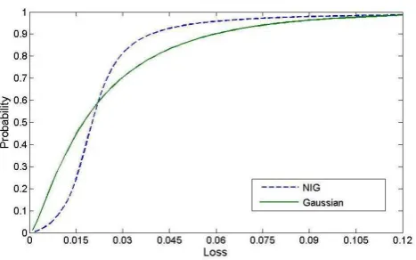
which cannot be simplified any further, the NIG distribution not always being symmetric6_.

Figure 4.3: In the chart the cumulative loss probability distributions obtained with the NIG and Gaussian copula have been compared in the lower tail.

6

4.1.2

α

-stable distributions

The α-stable is a flexible family of distributions described by Paul L´evi in the 1920’s and deeply studied by, e.g., Nolan [42, 43]. This distribution can be used efficiently for problems where heavy tails are involved and, as introduced by Prange and Scherer in [44], can be profitably used to price CDOs. Following Nolan7 _{we can define this family of distributions as follows:}

Definition 3 A random variable X is stable if and only if X := aZ +b, where 0 < α ≤ 2, −1 < β ≤ 1, a > 0, b ∈ R and Z is a random variable with characteristic function:

EeiuZ =

(

e−|u|α[1−iβtan(πα2 )(u)], if α6= 1

e−|u|[1+iβtan(π2)(u) ln|u|], if α= 1

(4.6)

Definition 4 A random variable X is α-stable Sα(α, β, γ, δ,1) if:

X :=

γZ+δ, if α6= 1

γZ+ (δ+β2_πγlnγ), if α= 1 (4.7)

where Z comes from the former definition.

The parametersγandδrepresent the scale and the location. In the sequel the simplified notation for a standard distribution Sα(α, β,1,0,1) :=Sα(α, β,1)

will be used to define the random variables. The family of stable distribu-tions8 _{includes widely used distributions, such as Gaussian, Cauchy or L´evi}

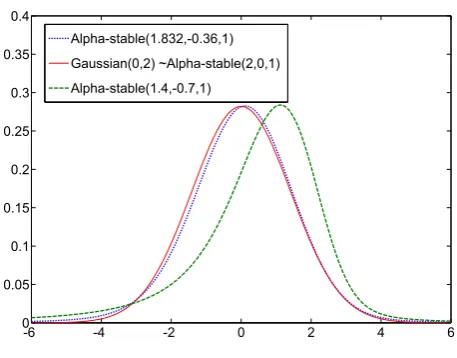
distributions (i.e. a Sα(2,0,1)∼Φ(0,2) as shown in figure 4.4).

From figure 4.4 it is possible to observe how decreasing the value for

α away from 2 moves probability to the tails and a negative β skews the distribution to the right, producing another distribution with a particularly fat lower tail.

We can apply this distribution to the simple factor model, where the com-mon and the specific risk factors Y and ǫi follow two independent α-stable

7

We would like to thank John Nolan for the α-stable distribution code provided. For further details visit http://www.RobustAnalysis.com.

8

Another definition of stable distribution can be the following:

Definition 5 _{A random variable X is stable if for two independent copies X}1, X2 and

two positive constants aandb:

aX1+bX2∼cX+d (4.8)

for some positive constant c and somed_∈R,

-6 -4 -2 0 2 4 6 0

0.05 0.1 0.15 0.2 0.25 0.3 0.35 0.4

Alpha-stable(1.832,-0.36,1)

Gaussian(0,2) ~Alpha-stable(2,0,1)

Alpha-stable(1.4,-0.7,1)

Figure 4.4: Examples of α-stable and Gaussian distributions. distributions:

Y _∼Sα(α, β,1),

and

ǫi ∼Sα(α, β,1),

this implies, using the properties of the stable distribution, that the firm risk factor follows the same distribution, i.e. Vi ∼Sα(α, β,1).

Given the i-th marginal default probability Fi(t), the default barrier Ki

is obtained inverting the relation P{Vi ≤ki}:

Ki =Fα−1(Fi(t)). (4.9)

The individual probability of default is:

p(t|y) = Fα

k−√ρY

√

1₋ρ

. (4.10)

Using 4.10 and the large pool approximation, given any x _∈ [0,1], the loss distribution as n_{→ ∞} can be written as:

G(x) = P{X _≤x_}= 1₋Fα

k₋

√

1−ρFα−1(x)

√_ρ

.

4.2

Stochastic correlation

The general model can be expressed as:

Vi = p

˜

ρiY + p

1₋ρ˜iǫi ≤ki, (4.12)

where Vi is a individual risk processY, ǫi, i= 1, ..., nare independent Φ(0,1)

and ˜ρi is a random variable that takes values in [0,1] and it is independent

from Y, ǫi. The latter independence assumption is particularly important as

conditioning upon ˜ρi the processesVi, i= 1, ..., nremain independent Φ(0,1)

and it is possible to calculate:

Ft(t) = P{Vi ≤ki}

= P{pρ˜iY + p

1₋ρ˜iǫi ≤ki}

= E[P{√ρY +p1₋ρǫi ≤ki|ρ˜i =ρ}]

=

Z 1

0 P{

√_ρY

+p1−ρǫi ≤ki|ρ˜i =ρ}dFρ˜i(ρ).

(4.14) We can then write Fi(t) = Φ(ki) and easily find the default threshold.

Under this model the individual probability of default can be calculated for ˜ρi ∈[0,1] :

pi(t|Y) = P{Vi ≤ki|Y}

= P{τi ≤t|Y}

=

Z 1

0

Φ

ki−√ρY

√

1−ρ

dFρ˜i(ρ).

(4.16) Following closely Burtschell et al. [14, 15], within this framework two dif-ferent specifications for ˜ρi are considered. In one case the correlation

ran-dom variable follows a binary distribution: ˜ρi = (1−Bi)√ρ+Bi√γ, where

Bi, i = 1, ..., n are independent Bernoulli random variables and ρ, γ ∈ [0,1]

Vi = q

((1−Bi)√ρ+Bi√γ)Y + q

1−((1−Bi)√ρ+Bi√γ)ǫi

= Bi

√

γY +p1−γǫi

+ (1−Bi)

√

ρY +p1−ρǫi

. (4.17) In this simple case the correlation ˜ρi can be either equal toρ or γ

condi-tioning on the value of the random variable Bi. The Bernoulli’s parameters

are denoted by pγ =P{Bi = 1}, pρ=P{Bi = 0}.

The expression for the individual default probability, conditioning on Y

and Bi and using tower property to integrate out Bi, leads to:

pi(t|Y) = P{τi ≤t|Y}=

1

X

j=0

P{τi ≤t|Y, Bi =j}P{Bi =j}

= pρΦ

_k

i−√ρY

√

1₋ρ

+pγΦ

_k

i−√γY

√

1₋γ

(4.18)

From 4.18 we can price CDO tranches calculating the loss distribution as in 2.26 for a homogeneous large portfolio:9

G(x) = P{pi(t|Y, Bi)≤x}

= P

Φ

k(t)−√ρ˜iY

√

1−ρ˜i ≤x = E P Φ

k(t)−√ρ˜iY

√

1₋ρ˜i ≤x

Y, Bi

= pρΦ

√

1₋ρΦ−1_(x)−k(t)

√_ρ

+pγΦ

√

1₋γΦ−1_(x)−k(t)

√_γ

.

(4.19)

This simple model can be very useful to replicate market prices through the use of two or three possible specifications for the correlation random variable. The ability to fit the market quotes much better comes from the fact that the joint default distribution is not a Gaussian copula anymore as described in section 2.2.1, but it is now a factor copula (see [15]). Particularly

9

A general case can be considered computing the distribution functionpi(t|Y) for each

under the LHP assumption it is quite effective to set up the correlation as follows:

˜

ρ=

 



ρ with, pρ

γ = 0 with, pγ

ξ = 1 with, pξ.

(4.20)

In this way we can combine an independence state whenγ = 0, that allows us to highlight the effect of the individual risk, with a perfect correlation state ξ = 1 for the latent risk. The idiosyncratic risk can be studied more effectively under independence assumption, since a default occurring does not result in any contagious effects. Therefore this kind of models can have a better performance during crisis periods when compared to a standard model10. The common risk can be controlled by increasing the probability of ξ = 1 and decreasing the probability associated with the other possible states of the random variable ˜ρ, thus moving probability mass on the right tail of the loss distribution and then rising the price for the senior tranches, which are more sensible to rare events.

A second approach to model stochastic correlation, proposed by Burtschell

et al.[15] admits a more sophisticated way to take into account the systemic risk. Instead of having a high correlation parameterξlike the previous model, we can set: ˜ρi = (1−Bs)(1−Bi)ρ+Bs, whereBs, Bi, i= 1, ..., nare

indepen-dent Bernoulli random variables and ρ∈[0,1] is a constant. The Bernoulli’s parameters are denoted by p=P{Bi = 1}, ps=P{Bs = 1}. This model has

a so called comonotonic state, or perfect correlation state occurring when

Bs= 1. The general model in 4.12 can be written as:

Vi = ((1−Bs)(1−Bi)ρ+Bs)Y + (1−Bs)( p

1−ρ2_(1−B

i) +Bi)ǫi

= ˜ρiY + q

1₋ρ˜i2ǫi. (4.21)

Under this specification of the model11_{, in analogy with the idea}

under-lying model 4.20, the distribution of the correlation random variable ˜ρi2, has

10

As reported by Burtschell et al.[15], following the downgrades of Ford and GMAC in May 2005, the higher idiosyncratic risk perceived by the market can be measured incorporating the idiosyncratic risk on each name and in particular on the more risky ones, i.e. the names with wide spreads.

11

Given ˜ρi = ρ we can easily verify that Corr[Vi, Vj] = E[Vi, Vj] = E[ρY +

p

(1−ρ2

)ǫi, ρY +

p

1−ρ2

ǫj] =ρ

2

E[Y2

] =ρ2

the following distribution: ˜ρi2 = 0 with probability p(1−ps), ˜ρi2 = ρ with

probability (1₋p)(1₋ps) and ˜ρi2 = 1 with probabilityps, which corresponds

to the comonotonic state.

The individual default probability can be found conditioning onY, Bi and

Bs:

pi(t|Y) =

1

X

l,m=0

P{τi ≤t|Y, Bi =m, Bs =l}P{Bi =m}P{Bs=l}

= p(1₋ps)Φ[ki(t)] + (1−p)(1−ps)Φ "

ki(t)−ρY p

1₋ρ2

#

+ps1{ki(t)≥Y}

= p(1−ps)Φ[Φ−1[Fi(t)]] + (1−p)(1−ps)Φ "

ki(t)−ρY p

1−ρ2

#

+ps1_{ki(t)≥Y}

= (1−ps) pFi(t) + (1−p)Φ "

ki(t)−ρY p

1−ρ2

#!

+ps1_{ki(t)≥Y}. (4.22)

This result can be used to find a semianalytical solution for the price of any CDO tranches (see [15]), or alternatively, conditioning on Y and BS,

can be used to approximate the loss distribution under the usual LHP as-sumption12_{. For the purpose of this work the analysis will be focused on the}

second approach. Givenx_∈[0,1], the loss distribution is then expressed by:

G(x) = (1−ps)

Φ

1

ρ

p

1−ρ2_Φ−1

x₋pF(t) 1−p

−k(t)

1_{x_∈A_}+1_{x_∈B_}

+ psΦ [−k(t)], (4.23)

where the notation has been simplified defining:

A=_{x_∈[0,1]_|pF(t)< x <(1₋p) +pF(t)_}, and

B ={x_∈[0,1]|x >(1−p) +pF(t)}.

Proof:

12

Using the tower property we have:

G(x) = P{p(t_|Y, Bs)≤x}

= E

"

P

(

(1−Bs) pF(t) + (1−p)Φ "

k(t)−ρY

p

1−ρ2

#!

+Bs1_{k(t)≥Y} ≤x

Y, Bs )#

.

(4.24)

Summing over the possible outcomes for Bs we have:

G(x) = (1−ps)E "

P

(

pF(t) + (1−p)Φ

"

k(t)−ρY

p

1−ρ2

# ≤x Y )#

+ psE

P

1_{k(t)≥Y_} ≤x Y

= (1−ps)E "

P

(

k(t)−ρY

p

1−ρ2 ≤Φ

−1

x₋pF(t) 1₋p

Y

)#

+psP{Y > k(t)}

= (1₋ps) Φ 1 ρ p

1₋ρ2_Φ−1

x₋pF(t) 1₋p

−k(t)

1_{x∈A}+1{x∈B}

+ psΦ [−k(t)]. (4.25)

In the formula above we recall that:

A={x_∈[0,1]|pF(t)< x <(1−p) +pF(t)}, and

B =_{x_∈[0,1]_|x >(1₋p) +pF(t)_}.

In step three we have used the fact that for 0≤ x < 1, 1_{k(t)≥Y_} if and

only if Y > k(t) and in step four that, assuming p <1 and ρ >0,

pF(t) + (1₋p)Φ

k_√(t)−ρY

1−ρ2

can take values between

(a) ifF(t)< x < (1₋p)+pF(t), then₋Y _≤ 1_ρp1₋ρ2_Φ−1hx−pF(t) 1−p

i

−k(t)

⇒P

pF(t) + (1−p)Φ

k_√(t)−ρY

1−ρ2

≤x Y = 1;

(b) x_≤F(t),

⇒P

pF(t) + (1₋p)Φ

k(t)−ρY

√

1−ρ2

≤x Y = 0; and

(c) x_≥(1−p) +pF(t),

⇒P

pF(t) + (1−p)Φ

k_√(t)−ρY

1−ρ2

≤x Y = 1.

This model can be used to adjust the probability in the upper part of the cumulative loss distribution, i.e. increasing ps raises the probability of

having credit events for all the names in the portfolio affecting the prices of senior tranches. Analogously increasing the idiosyncratic probability q

pushes probability towards the left part of the loss distribution, resulting in an increased risk for the junior holder and a lower risk for the senior investors. In the case of the mezzanine tranches the dependence is not always constant, generally not being monotone in correlation ρ.

4.3

Local correlation

The term “local correlation” refers to the idea underlying a model where the correlation factor ρ can be made a function of the common factor Y. This family of models belongs to the stochastic correlation class because, being

Y a random variable, the correlation factor ρ(Y) is itself stochastic. This approach was introduced by Andersen and Sidenius [4] with the “random factor loadings” (RFL) model and by Turc et al. [51]. The base assumption of these models is very interesting since it attempts to explain correlation through the intuitive relation with the economic cycle: equity correlation tends to be higher during a slump than during a growing economy period.

4.3.1

Random factor loadings

Vi =ai(Y)Y +vǫi+m ≤ki, (4.26)

whereViis a individual risk processY, ǫi, i= 1, ..., nare independentN(0,1),v

and m are two factors fixed to have zero mean and variance equal to 1 for the variable Vi.

The factor ai(Y) is a R → R function to which, following the original

model [4], can be given a simple two point specification like the following:

ai(Y) =

α if, Y _≤θ β if, Y > θ.

One can already observe the ability of this model to produce a correlation skew depending on the coefficient α and β: if α > β the factor a(Y) falls as

Y increases (i.e. good economic cycle) lowering the correlation amongst the names, while the opposite is true when Y falls below θ (i.e. bad economic cycle). In the special case α = β the model coincides with the Gaussian copula, but in general both the individual risk process Vi Gaussian and the

joint default times do not follow a Gaussian copula.

The coefficients v and m can be easily found solving for E[Vi] =E[ai(Y)Y] +m = 0,⇔E[ai(Y)Y] =−m

Var[Vi] = Var[ai(Y)Y] +v2 = 1),⇔Var[ai(Y)Y] = 1−v2

then we can calculate the values for m and v:

E[ai(Y)Y] = E[αY1{Y≤θ}+βY1{Y >θ}Y]

= ϕ(θ)(₋α+β), (4.27) and

E[ai(Y)2Y2] = E[α2Y21_{Y≤θ}+β2Y21{Y >θ}Y]

= α2(φ(θ)₋θϕ(θ)) +β2(θϕ(θ) + 1₋φ(θ)), (4.28) from which13 _{the solutions are:}

13

In the equations 4.27 and 4.28 was used that E[1_{a<x≤b}x] = 1_{a≤b}(ϕ(a)−ϕ(b))

E[1_{a<x≤b}x2

] = 1_{{α≤b}(Φ(b)−Φ(a)) +}1_{{a≤b}(aϕ(a)−bϕ(b)), see [4] Lemma 5 for a}

m=ϕ(θ)(α₋β), and

v =p

1₋Var[ai(Y)Y].

As already recalled,Vi are in general not Gaussian in this model, thus the

calculation to find the individual default probability and the default threshold changes. The conditional default probability can be calculated as follows:

pi(t|Y) = P{Vi ≤ki|Y}=P{τi ≤t|Y}

= PαY1_{Y≤θ} +βY1{Y >θ}Y +ǫiv+m≤ki|Y

= P

(

ǫi ≤

ki− αY1_{Y_≤θ_}+βY1_{Y >θ_}Y −m v Y ) .(4.29) Integrating out Y, and using that ǫi is a standard Gaussian under this

simple specification of the model, the unconditional default probability for the i-th obligor is:

pi(t) = E "

P

(

ǫi ≤

ki− αY1_{Y_≤θ_}+βY1_{Y >θ_}Y −m v Y )# = Z θ −∞ Φ

ki−αY −m

v

dFY(Y)

+

Z ∞

θ

Φ

ki−βY −m

v

dFY(Y).

(4.30)

From this integral it is straightforward to calculate the default threshold

ki numerically.

Alternatively, using that Y follows a Gaussian distribution, and using some Gaussian integrals14a solution of the 4.30 can be found using a bivariate

14

For a proof of the following Gaussian integrals see [4] lemma 1:

Z ∞

−∞

Φ [ax+b]ϕ(x)dx= Φ

b

√

1 +a2

Z c

−∞

Φ [ax+b]ϕ(x)dx= Φ2

b

√

1 +a2, c; −a

√

1 +a2

Gaussian cdf15_:

pi(t) = P{Vi ≤ki}

= Φ2

θ₋m

√

v2_+α2, θ;

α

√

v2_+α2

+ Φ

"

θ₋m

p

v2_+β2

#

− Φ2

"

θ₋m

p

v2_+β2, θ;

β

p

v2_+β2

#

.

(4.32) Assuming a large and homogeneous portfolio, given any x _∈ [0,1] it is possible to find a common distribution function G(x) for pi(t|Y) as n → ∞

using, as before, the result stated in Vasicek [52]:

G(x) = 1−P(X > x)

= 1₋Pa(Y)Y _≤ki−vΦ−1[x]−m

= 1₋(P{αY _≤Ω(x), Y _≤θ_}+P{βY _≤Ω(x), Y > θ_}) = 1−

Φ

min

Ω(x)

α , θ

+1_{θ<Ω(x)

β }

Φ

Ω(x)

α

−Φ [θ]

(4.33)

where Ω(x) :=ki−vΦ−1[x]−m.

4.4

Stochastic correlation using normal

in-verse Gaussian

This model represents an attempt to shape the correlation skew and then the market prices combining two of the solutions presented in the previous subsections. The stochastic correlation model, as presented in 4.12, can be efficiently used with NIG distributions for the systemic and the idiosyncratic risks factors Y, ǫi, i = 1, ..., n,16 instead of normal random variables. This

15

Depending on the quadrature technique used 4.30 can be solved directly more effi-ciently than 4.31, which involves a bivariate Gaussian.

16