Compatibility in Tax Reporting

Munich Personal RePEc Archive

Compatibility in Tax Reporting

Lipatov, Vilen

European University Institute

February 2006

Compatibility in Tax Reporting

Vilen Lipatov

Abstract

We consider corporate tax evasion when business partners have di¤erent attitudes towards aggressive tax accounting. There are costs of uncoordinated

tax reports, both in terms of catching inspectors’ attention and running ac-counts. If these costs are small, there exist a unique stable Nash equilibrium of

the game between the tax authority and a population of heterogeneous …rms. In this equilibrium, the relation between compatibility costs and compliance is

non-monotonic and depends on the curvature of auditing function. However, compatibility costs reduce non-compliance in low cheating regimes and may enhance it when many …rms are cheating. This provides one rationale for

de-veloping countries to be cautious with employing re…ned auditing schemes and for developed countries to promote complicated accounting procedures.

JEL Classi…cation: H26, H32

Keywords: tax evasion, compatibility, coordination, business partners, tax ac-counting

1

Introduction

Recent years have seen a surge in research on tax evasion of …rms. The interest was aroused by an observation that …rm adds new dimensions to the problem over and above standard gambling and cat-and-mouse1 _{approaches. Firstly, a …rm is not a}

I am grateful to Chaim Fershtman, Massimo Motta, Rick van der Ploeg, Karl Schlag and par-ticipants of workshops at European University Institute, Tinbergen Institute, Hannover University; Labsi and Ruhr Graduate School Conferences for the comments on an earlier version of this paper entitled "Tax Evasion and Coordination".

y_{Frankfurt University, Grüneburgplatz 1, 60323 Frankfurt am Main, Germany.}

1_{The term is borrowed from Cowell (2006) and refers to the modeling of evasion as a game}

single decision maker and has its own agency problem, as stressed by Crocker and Slemrod (2005). Second, the interaction between …rms can be important for the general outcome, as Bayer and Cowell (2009) and Sanchez (2006) point out, although Lipatov (2008) shows that the interaction matters in games with individual taxpayers as well.

Even in the simplest cases successful hiding of information from tax authority re-quires coordinated action of at least two parties. In sophisticated evasion (tax evasion that requires certain expertise and involves intricate manipulation of accounts), there may be multiple parties as well as substantial costs of making accounts consistent and looking good at super…cial checks of tax authorities. In the US, Sarbanes-Oxley act of 20022 _{has made these costs even higher}3_.

The act is largely seen as a response to corporate scandals which were undermining con…dence in the American securities market. The congress has designed it to promote transparency: increased disclosure becomes mandatory, corporations are required to install new board oversight and internal controls, investors are promised to be given better information. In 2003 companies shelled out an average of $16 million on Sarbox compliance, up 77 percent from the year before. An article in the Economist 2004 devoted to the controversy of this act was entitled “404 tons of paper” referring to the aspect of compatibility costs that are in the spotlight of our paper.

The other aspect of costs to coordinate are di¤erences in the tax reports that should be similar a priory. In case of business partners, the tax authority observes transactions and can audit both partners, having some idea of how correlated their incomes are. It is well known in the profession that the tax audits are not random. First, the taxpayers are divided in homogenous auditing classes. Second, within each class the tax authority may receive some signals that a given report is suspicious. One of such signals is a discrepancy in the reports of business partners. The importance of coordination in tax reporting is also con…rmed experimentally by Alm and McKee (2004).

The counter-checking of reports is a standard procedure for some taxes. For VAT, this particularly makes sense, as a part of the tax that is paid by one party is then rebated by the other. Das-Gupta and Gang (2001) model the matching of purchase and sales invoices explicitly. They conclude that cross-matching can induce truthful

2_{The following information about the act is taken fromhttp://www.fmsinc.org/cms/?pid=3253} 3_{The data availability requirements that are also part of costs can be checked at}

reporting, but distorts purchase and sales decisions. In Russia the auditing of one …rm involves checking accounts of the …rms that are transacting with it, as described e. g. in Sumina (2006).

McIntyre (2005) writes that most of the modern sheltering schemes undermine the basic principle of tax law: a tax deductible item of one taxpayer is a part of taxable income of the other. The evasion opportunity arises when one …rm deducts some payments made to the other …rm, but this other …rm is not taxable, e. g. it is an o¤-shore company. This kind of evasion looks simple in principle, but requires sophisticated organization and coordination not to be obvious. In turn, the detection of such evasion requires counter-checking of the reports provided by business partners. In Russia, the mechanism of evasion is similar, though the schemes are usually blunter: the accounting specialists register a lot of …ctitious …rms some of which just do not pay taxes and disappear.

We look here at a long run situation in an economy where …rms exercise trans-actions with each other. Before entering the industry, a …rm has to decide whether to adopt aggressive attitude towards tax reporting or to stay on the compliant side. This choice of accounting standard is analogous to the choice of a computer operating system in its compatibility aspect. That is, while operating together, the …rms with di¤erent accounting machineries incur higher transaction costs than the …rms with similar accounting procedures do.

If a …rm decides to be aggressive, it hires a tax evasion specialist who arranges accounts for a certain fee4_{. A compliant …rm manages accounts itself. After the} accounting policy has been adopted, the …rms start operating and transacting with other …rms. Finally, the …rms get pro…ts and report them to a tax authority. The tax authority observes the transacting …rms and decides on the auditing intensity.

Thus, in our economy the …rms face two kinds of costs in addition to standard costs and bene…ts of evasion. The …rst type is compatibility costs, which have to be borne every time there is a transaction between …rms with di¤erent accounting standards. These are related to the adjustment of accounts for di¤erent kinds of …rms: e. g., the aggressive and complying …rms often prefer transactions to be re‡ected in the books at di¤erent time points or at di¤erent locations5_{. The second type is endogenous} costs, which arise every time the tax authority sets unequal probability of auditing

4_{We treat the specialist as a passive player here. Her optimization problem is analysed in Lipatov}

(2008).

for the cases of observing similar and di¤erent reports of the two …rms whose income is known to be correlated.

The endogenous costs are also present in Sanchez (2006). The di¤erence of his paper from our approach is not only in the lack of compatibility costs, but also that he considers tax authority with ability to commit. This is well explained by di¤erent ideas underlying the two papers: whereas we consider long-run equilibrium, Sanchez concentrates on the short-term with the aim of constructing auditing rule that minimizes mistakes of the tax authority (in sense of auditing the honest and not auditing cheaters). Furthermore, whereas Sanchez describes the situation in a homogenous auditing class, assuming perfect correlation of income and uncertainty about the auditing rule, we consider a pair of …rms with imperfectly correlated income. The paper by Bayer and Cowell (2009) stands even further from us: it looks at the e¤ect of auditing on joint decision of competing …rms to evade and to produce. Though their main result, the desirability of non-…xed auditing rule, survives in our setup, we consider …rms that are partners rather than competitors, and we focus on the e¤ect of compatibility costs rather than auditing rules. Crocker and Slemrod (2005) go inside a …rm, whereas we treat it as a decision making unit.

In our model, the tax authority has no ability to commit. Firstly, this has a natural appeal for the long run modeling. Secondly, though the auditing rules are often announced by the tax authorities, there is no means to establish whether they are actually followed.

The main result of the paper is equilibrium characterization: We …nd out that equilibrium cheating and auditing di¤er substantially from the approach disregarding transactions among the …rms, even if the compatibility costs are small. When evasion is small, the share of cheating …rms as well as the auditing probability is likely to be overestimated, if the coordination of tax reports is not taken into account. In case of popular misreporting, both the share of non-compliers and the auditing probability may be underestimated. It is worth noting that the auditing probability in our setting varies with the reports combination, making comparison with uniform auditing probability of the representative case di¢cult in principle.

strategic reaction of the tax authority. The total e¤ect of any parameter on the endogenous variables is then in‡uenced by the sum of the three e¤ects identi…ed.

For a large class of auditing technologies, we …nd that compatibility costs decrease cheating and auditing when only few …rms are underreporting and increase them in case evasion is popular. The correlation of pro…ts has a similar e¤ect. In both instances, with coordination cost ascent the more popular strategy becomes more attractive; hence more …rms choose it in equilibrium. Somewhat surprisingly, but following exactly the same logic, improvement in auditing technology and …nes reduce cheating in low evasion regimes and enhance it in high evasion regimes.

The auditing probability in our model can be positively a¤ected by the amount of …nes, unlike in representative case. This becomes possible because the direct e¤ect of larger …nes to make auditing more attractive may overplay the indirect e¤ect coming through the reduced cheating. Finally, the e¤ectiveness of …ne always decreases as a result of an increase in compatibility costs.

We also shed some light on the mechanism of evasion game when compatibility matters: we show that correlation of pro…ts solely generates the di¤erence in auditing probabilities. The compatibility costs alone change equilibrium cheating and auditing, but leave the latter independent from the report con…guration.

The rest of the paper is structured as follows. The model setup is presented in the next section, followed by the description of equilibrium structure. Section four is devoted to the discussion of the results for the mixed equilibrium. Section …ve looks at an example of particular auditing technology. Conclusion is followed by appendix with derivations of equilibria and results.

2

Evasion game

2.1

Single …rm benchmark

Let us start with the case when there are no transacting pairs and no compatibility costs. A single …rm decides whether to evade its pro…t, facing the tax authority that can perform auditing. We use the approach of Graez, Reinganum and Wilde (1986) in this benchmark, with a convex rather than linear cost function for auditing.

function

f(x) =

(

if x= 1 if x= 0 :

Second, the high pro…t …rms decide whether to submit a high report H = (be honest) or a low reportL= 0 (cheat).

The tax authority does not audit high reports and exerts e¤ort a in auditing low reports. A continuous function a : [0;1) ! R+ is a mapping from detection

probability de…ned on the unit interval to the auditing e¤ort de…ned for non-negative real numbers. The inverse function determines detection probability from the e¤ort

p:R+! [0;1). We assume that the …rms can never be detected with certainty, and

zero e¤ort results in zero detection probability p(0) = 0. The low report is honest with probability ₁ 1 _+q and not with the complementary probability, where q is the probability that high pro…t …rm is cheating.

The authority is maximizing its expected revenue ₁ q_+q p(a) (1 +s)t a, the high income …rm - its expected pro…t p(a) (1 +s)t . Here s is a surcharge rate for being caught, t is a tax rate. In equilibrium with positive detection probability FOC for the tax authority p0

(a ) (1 +s)t = 1_q + 1, and indi¤erent condition for the …rm is . Hence equilibrium e¤ort is

p(a ) = 1 1 +s

and equilibrium evasion probability is

q = 1 1

p0 _{p 1} 1

1+s (1 +s)t 1

:

Su¢cient conditions for the existence of such an equilibrium: p is strictly increas-ing and strictly concave, p0

p 1 1 1+s >

1

(1+s)t . The latter actually ensures mixed

2.2

Two transacting …rms

Recall the story behind our model, presented in the introduction. Firstly, the …rms choose their accounting standards. Second, the …rms are matched according to some rule. Third, the …rms draw pre-tax incomes from participating in a match. The second and third stages may repeat a number of times. Fourth, the …rms summarize the realized income and submit a tax report. Finally, the tax authority audits the tax reports of some …rms (and all its partners).

To make the analysis as simple as possible while preserving the coordination as-pect, we make the following simplifying assumptions: (i) each …rm meets only one transacting partner; (ii) each …rm makes only one transaction; (iii) the aggressive …rm does not report truthfully. Under these assumptions the game above is equivalent to the following 3 player game.

2.2.1 The setup

Consider a simultaneous game between two risk neutral …rms and a tax authority. The …rst move is made by the …rms. They decide whether to adopt aggressive accounting policy and pay a price b per evaded euro for it, 0 b < t, or to use compliant accounting that comes at a cost normalized to zero.

The second move is made by the nature that assigns a type to each of the two …rms: high pro…t h = or low pro…t l = 0. We assume now that the pro…ts are correlated with the correlation coe¢cient r;0 r <16_{. We do not consider negative} correlation, as our …rms are cooperating rather than competing. The joint distribution of two types in a match is given by the following density function:

f(x; y) =

8 > > <

> > :

; if x=y = ; ; if fx; yg=f0; g;

1 2 + ; if x=y = 0:

where := 2_{+ (1 )r; 2[} 2_{; ).}

After the pre-tax pro…t is realized, the …rms submit their reports according to the procedure they chose in the …rst stage. Namely, the low income …rm submits a

6_{We have also analyzed the case whenr= 1, but since this is not likely to happen in reality, we}

low report and gets a payo¤ normalized to 0, if its partner has the same accounting standard, and c, if it has a di¤erent standard. The high income …rm submits a high report H = (be honest) if chose compliant policy or a low report L = 0 (cheat) if chose aggressive policy. Each …rm of type h (high pro…t) gets ex interim expected payo¤ (before the coordination costs c) of u(i; j), where i is its own report and j is a report of its partner:

u(L; L) = p aLL _{(1 +s)t b ;} u(L; H) = p aHL _{(1 +s)t b ;} u(H; H) = u(H; L) = (1 t):

Ex ante expected pro…t is then the following. If a …rm decides to use aggressive accounting,

u(A) = (qu(L; L) + (1 q)u(L; H)) + ( )u(L; L) + (1 ) 0 (1 q)c:

Here the event when both the …rm and its partner get high pro…t de…nes the …rst term, the event when the …rm gets high pro…t and its partner gets a low one de…nes the second term. The third term contains the payo¤ in the event of our …rm getting low pro…t, normalized to zero. In any event we have to subtract coordination cost c

in case our aggressive …rm is matched with the compliant one, and that is what the last term takes care of.

If a …rm decides to use compliant accounting, it is

u(C) = (qu(H; L) + (1 q)u(H; H)) + ( )u(H; L) + (1 ) 0 qc:

The terms are similar: both …rms getting high pro…t, only the compliant …rm getting high pro…t, and the compliant …rm getting low pro…t.

The third move is by the tax authority, which chooses an auditing e¤ort a 2R+

conditional on the reports observed: a(LL) (two low reports), a(HL) (a low and a high report in any order),a(HH)(two high reports). The tax authority gets expected revenue of p(a) (1 +s)t afrom each cheater it audits and the revenue t afrom each honest report it audits.

Compared to the case of two low reports, it needs a half of resources to provide the same auditing probability if one of the reports is high. Thus, we do not consider the case in which coordinated evasion requires more e¤ort to discover than uncoordinated does.

We choose the simultaneous formulation rather than a sequential one, because we do not want to consider a particular industry structure or a relation between an entrant and an incumbent. Our goal is to characterize the economy where two …rms from di¤erent populations (again, think of buyers and sellers) meet to play a coordination game. Even more, since the decisions are long-term, they become a property of the …rms, so that they can be characterized as evaders or honest. In this way, the Nash equilibria of the simultaneous game show us where these populations could converge to.

2.2.2 Optimization problem of the tax authority

The tax authority observes the match. Recall that we denote with lower-case letters the pro…ts, and with uppercase the reports. We have then the following pro…t -report table

total HH HL LL

hh (1 q)2 2 q(1 q) q2

hl 2 ( ) 0 2 ( ) (1 q) 2q( )

ll 1 2 + 0 0 1 2 +

which represents the measures (or shares) of taxpayer pairs reporting incomes given by the column entries, while actually receiving incomes given by row entries.

The following lemma characterizes the best response of the tax authority in this case.

Lemma 1 In the tax evasion game above the best response of the tax authority a(q)

to the …rms cheating with probability q 2(0;1] is implicitly de…ned by:

aHH = 0; (1)

p0

aHL(q) = q+

q(1 +s)t ; if q q

0

HL; (2)

p0

aLL_{(q) =} q2+ 2q( ) + 1 2 +

( q2_{+q( )) (1 +s)t} ; if q q 0

LL; (3)

aHL_{(q) = 0; if q < q}0

HL;a

LL_{(q) = 0; if q < q}0

The proof is left to the appendix A,q0

HL andq0LLare also de…ned there. Obviously,

observing two high reports the tax authority does not audit them. Observing di¤erent reports in a match, the authority audits the low one with probability determined by the e¤ortaHL_{(q). When two low reports are observed, the optimal auditing e¤ort is}

given byaHL_(q).

Note that the two e¤orts (and corresponding probabilities) are only equal, when

r= 0, that is the report of one …rm does not contain any information about the pro…t of the other …rm. With r > 0 we have aHL_{(q) a}LL_{(q), which is quite intuitive:}

di¤erent reports indicate possible cheating, so it makes sense to audit them more.

2.2.3 Equilibria

Before stating the result it is useful to introduce the following terminology:

De…nition 1 We call an equilibrium of our game full cheating, if all the …rms are

submitting low (zero) reports in this equilibriumq = 1; we call an equilibrium

full honesty, if all the high income …rms submit high reports q = 0.

The proposition 1 characterizes the equilibria arising in case of correlated draws. We denote the equilibrium values of cheating probability withq and of auditing e¤ort with a .

Proposition 1 In the tax evasion game with two transacting …rms

(i) There exists a symmetric evolutionary stable equilibrium with q implicitly de…ned by

(t b) (1 2q )c= ( (1 q ))p aLL_{(q ) + (1 q)p a}HL_{(q ) (1 +s)t ;}

(5)

aHH _{= 0, a}HL _=aHL_{(q ),a}LL _=aLL_{(q )as given by (1), if the compatibility}

costs are small and

(t b) 1 2qLL0 c > 1 q0LL p a HL

q0LL (1 +s)t ; (6)

where q0

LL re‡ects auditing technology and is de…ned in the appendix.

(ii) There exists a symmetric evolutionary stable equilibrium with q implicitly de…ned by

aHH _{= 0, a}HL _{= a}HL_{(q ), a}LL _{= 0, if the compatibility costs are small and}

(6) does not hold7_.

(iii) If (t b) c 0, there exist a full honesty equilibrium with q = 0; a 0.

(iv) If (t b) +c p aLL_{(1) (1 +s)t , there exist a full cheating}

equi-librium, and q = 1; aHH _{= 0,a}HL _=aHL_(1),aLL _=aLL_(1).

The proof of the proposition is left to appendix B. The structure of equilibria is very intuitive: for small compatibility costs (how small they should be depends on the auditing technology) there is a unique stable mixed equilibrium, as in a standard game without coordination issues. A small quali…cation here is that it takes a di¤erent form depending on whether consistent low reports are audited (i) or not (ii).

With larger compatibility costs, multiple equilibria may arise. More importantly, full honesty and full cheating may become equilibrium, as with everybody around being honest it is too costly in terms of compatibility to use aggressive accounting and visa versa. Whereas only the magnitude of the compatibility costs (relative to the evasion bene…ts) decides whether there exist full honesty equilibrium (iii), the auditing technology also plays a role in determining the existence of full cheating equilibrium (iv).

3

Discussion of the results

3.1

Summary

Since we believe that the exogenous coordination costs are relatively small, we can concentrate on the regions of parameter values where a mixed equilibrium exists. As it has been already noted, the probability of auditing for dissonant reports is higher than that for the similar reports as long as r > 0. A further breakdown of the compatibility costs propagation mechanism is represented in the table below:

c= 0; r= 0 c >0; r= 0 c= 0; r >0

p (LL) t b

(1+s)t p p

0 1 q +1

q (1+s)t p p

0 1 q 2

+2q ( )+1 2 +

( q 2_{+q ( ))(1+s)t}

p (HL) t b

(1+s)t p p

0 1 q +1

q (1+s)t

t b

(1+s)t

7_{The equilibria characterized in (i) and (ii) are also unique under the conditions speci…ed in the}

From this table we see clearly that the di¤erential auditing probability is generated from some correlation even in the absence of exogenous compatibility costs. On the other hand, only exogenous costs cshift equilibrium cheating probability even in the absence of auditing intensity di¤erential: The following expression determines the share of aggressive …rms with independent draws.

(t b) (1 2q )c= p p0 1 q + 1

q (1 +s)t (1 +s)t : (8)

Thus, the two channels of the compatibility costs can be clearly separated.

The following remark shows how the expected payo¤ of the …rmsI depend on the compatibility costs. The payo¤ is easy to compute because in the mixed equilibrium the …rms a ex ante indi¤erent between aggressive and compliant accounting.

Remark Compatibility costs put a burden on the …rms unless there is a full honesty:

I = (1 t) q c.

3.2

Comparative statics

Firstly, we are interested in how the equilibrium value of cheating depends on the compatibility costs. For q > q0

LL, from (5) we have

(1 2q )dc=Qdq; (9)

Q:= p a

HL _{p a}LL _{( (1 q ))p}0

aLL _aLL q

(1 q )p0

aHL _aHL q

!

(1 +s)t + 2c:

(10)

On the lhs we see the direct e¤ect ofcon the costs of evasion: When there are more compliant …rms (q < 1=2), the e¤ect is positive, as there is a higher chance to meet a compliant …rm and incur the compatibility costs. Otherwise (q >1=2), the e¤ect is negative, as there is a higher chance to meet a …rm with aggressive accounting.

e¤ect). The second term re‡ects the negative e¤ect of q on the attractiveness of evasion through raising auditing probability for both types of the reports (“auditing change” e¤ect). The third term is positive and re‡ects the increase in bene…ts from evasion through saving on compatibility costs (“saving” e¤ect).

Thus, the total indirect e¤ect is ambiguous. Note that this is true not only for compatibility costs, but for any parameter a¤ecting q, since it is actually change in

q itself that either increases or decreases attractiveness of evasion depending on how responsive the auditing probability is. This in turn depends on the curvature of the auditing function (we see p0

(a)directly in (9), in appendix we show that aq depends on p00

(a)). As p0

(a) is decreasing in q with @2_p0

(a(q))=(@a@q) < 0, the e¤ect of the auditing change is most likely to outweight other e¤ects for small q, and visa versa. Because of strict monotonicity and p(+1) 1, auditing functions satisfy

p0

(+1) = 0. So, the auditing change e¤ect evaporates for large q, and the total e¤ect becomes positive.

For the class of functions with p0

(0) = +1, q0

LL = qHL0 = 0 and the auditing

change e¤ect grows unboundedly large at zero, whereas the lhs is bounded, so the total e¤ect is certainly negative. Thus, for such functions there is a threshold value of equilibrium share of cheaters qc_{, below which the total indirect e¤ect is negative}

(and hence dq =dc < 0 for q < minf1=2; qc_{g), and above which the total indirect}

e¤ect is positive (and hence dq =dc <0 for q >maxf1=2; qc_g).

We also note that the di¤erential probability e¤ect is reinforced by pro…t correla-tion more than the auditing change e¤ect, so the total is more likely to be negative with lower correlation. At the extreme of independent draws we shall have

Q= p0

(a)aq(1 +s)t + 2c;

which is negative, if compatibility costs are small.8

If the equilibrium is at the intersection when only inconsistent reports are audited, that is q0

HL < q < q0LL, we have

(1 2q)dc=Q0dq (11)

Q0 := p aHL _{(1 q)p}0

aHL _aHL

q (1 +s)t + 2c

We can see the play of all e¤ects described above also here. The di¤erential probability is represented by p aHL _{and the auditing change e¤ect is weakened,}

8_{For su¢ciently large compatibility costs the total e¤ect is positive, but this is most likely to be}

because the similar reports are not audited. We know that close to q0

HL the total

e¤ect is negative, as p aHL_(q0

HL) = 0. With higher q the di¤erential probability

e¤ect kicks in and the auditing change e¤ect is less pronounced, so that the total may even change its sign.

Second, we are interested in the e¤ect of correlation on the equilibrium share of …rms that use aggressive accounting. For an equilibrium with non-zero auditing of both report combinations9_{, we have}

Dd =Qdq; (12)

D:= ( (1 q ))p

0

aLL _aLL_{+ (1 q )p}0

aHL _aHL

+ p aHL _{p a}LL _{(1 q )}

!

(1 +s)t (13)

The direct e¤ect of the correlation on the costs of evasion is always positive (the last term inD). It increases in the probability di¤erential and the share of compliant …rms. Intuitively, with higher correlation di¤erent reports are more likely, other things being equal. And since di¤erent reports are more likely to be detected and punished than similar, expected …ne increases in pro…t correlation. The indirect e¤ect of the correlation through auditing probability is represented by the …rst two terms in the expression forD. The …rst term is a negative e¤ect through the decrease in auditing of similar reports (aLL _{<0), the second term is a positive e¤ect through the increase}

in auditing of di¤erent reports (aHL _>0).

Here we can observe that for small q the negative e¤ect becomes small, whereas for largeqthe positive e¤ects vanish. The total e¤ect of correlation onqdepends then on the indirect e¤ect discussed at length above. For example, for auditing functions satisfying Inada conditionsdq =dr <0 for both very small and very largeq .

Third, we would like to see how an improvement in auditing technology a¤ects the equilibrium. Consider a new auditing technologyp1_{(a) = kp(a); k >0. Then}

Kdk =Q1dq; (14)

K := ( (1 q )) p a

LL_{(q ) +kp}0

aLL _aLL k

+ (1 q)p aHL_{(q ) +kp}0

aHL _aHL k

!

(1 +s)t : (15)

where Q1 _{is a correspondingly adjusted version of Q that takes into account k. As}

expected, the direct e¤ect of an improvement in auditing on the costs of evasion is positive: the same e¤ort of the tax authority results in higher expected …ne for a …rm.

The indirect e¤ect is negative: with more e¤ective auditing the optimal auditing e¤ort is reduced, so the expected …ne goes down as well. The total e¤ect K depends on the size ofp00

(a): If p(k) is concave, the direct e¤ect is higher than the indirect one, so the total e¤ect of an improvement in auditing on the evasion costs is positive; the opposite is true for convex p(k).

The e¤ect through equilibrium cheating Q1 _{is not a¤ected much, as both}

di¤eren-tial probability and auditing change e¤ects are ampli…ed to the same extent, only the compatibility e¤ect becomes relatively less important. Then with Inada conditions and positiveK,dq =dk < 0for q < qc_{, dq =dk >0 for q > q}c_{, that is improvement}

in auditing technology reduces cheating in low evasion regimes and enhances it in high evasion regimes.

Fourth, we look at the …ne. In our model the cheating is not necessarily decreasing in the surcharge rate s. The deterrence e¤ect depends again on whether an increase inq curbs or boosts bene…ts of evasion, i.e. on the sign of Q:

( (1 q ))p aLL_{(q ) + (1 q)p a}HL_{(q ) t ds=Qdq: (16)}

With Inada conditions that meansdq =ds < 0for q < qc_{, dq =ds >0 for q > q}c_.

We de…ne the measure of e¤ectiveness of the …ne as the absolute value of the derivative of the equilibrium cheating dq_ds . We immediately see that this mea-sure is decreasing in compatibility costs, so the …nes loosen their grip with higher costs in our equilibrium. This is important to have in mind while formulating a tax/enforcement/accounting policy.

4

Example

We take a function a(p) = kln(1 p) from Reinganum and Wilde (1986). The inverse function is p(a) = 1 e ak. k is a detection di¢culty parameter: the higher

it is, the more e¤ort is required to support a given detection probability.

From Lemma 1, using the functional form for the auditing technology, we can write

aHL(q) = kln k q+

q(1 +s)t ; q > q

0

HL; (17)

aLL(q) = kln k q

2 _{+ 2q( ) + 1 2 +}

( q2_{+q( )) (1 +s)t} ; q > q 0

The two thresholds are

qHL0 =

= 1

(1 +s)t 1;

q0LL =

( ) ((1 +s)t 2) +

q

( ) ((1 +s)t 2)2+ 4 ((1 +s)t 1) (1 2 + )

2 ((1 +s)t 1) ;

assuming(1 +s)t >2.

From Proposition 1 we have

(t b) (1 2q )c= ( (1 q))k

q (19)

1 q

q k

q + 1

q + 1 + ((1 +s)t k): (20)

This is a third degree polynomial, so we have to solve it numerically. For the com-plementary case

(t b) (1 2q)c= (1 q) (1 +s)t k 1 +

q ;

Full cheating condition isc+k > (b+st), full honesty condition is (t b) < c.

4.1

Parameterization

In the following we calibrate our parameters to the values common in the literature. We want to see how at plausible parameter values the compatibility costs a¤ect equi-librium cheating and auditing quantitatively. To do this, we shall …rstly explain the choice of parameters. Secondly, we de…ne two benchmarks according to how wide-spread evasion is: popular cheating (q= 0:6) featuring developing countries and rare cheating (q= 0:2) characterizing developed world. Finally, we look at how the cheat-ing and auditcheat-ing probabilities as well as tax revenue are changcheat-ing for each of the benchmarks.

Since the literature before us did not consider compatibility costs explicitly, we leave them free. We take the values of most parameters directly from Lipatov (2008), as we follow the same logic there: s = 0:8; t = 0:3; = 0:5. Fixing correlation at

With these parameter values our thresholds are

qHL0 = 0:075758;

qLL0 = 0:47118

We see that for low evasion regimeq0

HL < q < qLL0 , for high evasion regimeq > qLL0 .

We …x b = 0:03 in high evasion equilibrium to feature the widespread Russian 3% rule for the evasion service and (somewhat arbitrarily) b = 0:2 in low evasion equilibrium.

4.2

Low evasion regime

For the low evasion regime we can calibrate auditing e¤ectiveness as

k = ( 10 (b t) + 10t (q 1) (s+ 1))

1

q ( ) + 1 (q 1)

= 1:4

and we have c <0:5 as a condition for non-existence of full cheating or full honesty

equilibria.

Share of …rms with aggressive accounting

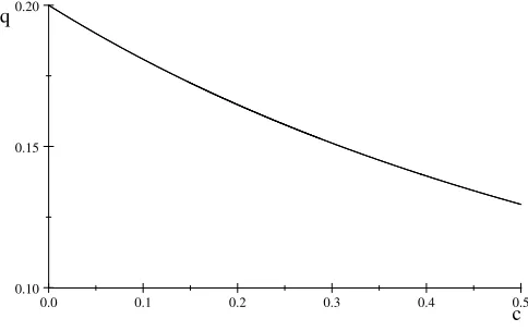
Fixing the parameters, we get the following picture:

0.0 0.1 0.2 0.3 0.4 0.5

0.10 0.15 0.20

c q

Figure 1. The e¤ect of compatibility cost con

evasion share q, low evasion regime.

share (from 20% to about 13%). We see that the costs have a substantial disciplining e¤ect on tax reporting in low cheating regime.

0.4 0.5 0.6 0.7

0.0 0.1 0.2 0.3 0.4

r q

Figure 2. The e¤ect of pro…t correlation r on evasion

share q, low evasion regime, c= 0:1.

From …rgure 2 we can see that correlation has a similar e¤ect on the equilibrium share of cheating. An increase in correlation from 40% to 60% drives cheating down from 28% to 13%.

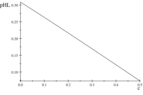
Auditing probability

The auditing probability (only di¤erent reports are audited) is plotted on the …gure 3:

0.0 0.1 0.2 0.3 0.4 0.5

0.10 0.15 0.20 0.25 0.30

c pHL

Figure 3. The e¤ect of compatibility cost con

auditing probability pHL_{, low evasion regime.}

e¤ect: an increase in compatibility costs from zero to0:5causes auditing probability to drop from above 30% to less than 10%). This is a very substantial e¤ect, so the cost savings associated with decreased auditing could be used to …nance introduction of higher compatibility costs.

The e¤ect of pro…t correlation on auditing probability is also positive in our pa-rameterization. In general, from Lemma 1 we know that @pHL_{=@r > 0, and since} dpHL_{=dq >0 and from …gure 2 dq=dr < 0, we have an ambiguous sign for dp}HL_=dr.

For our example, the direct e¤ect outweighs the one through the compliance, so the total e¤ect is positive.

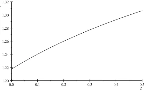
Tax revenue

0.0 0.1 0.2 0.3 0.4 0.5

1.20 1.22 1.24 1.26 1.28 1.30 1.32

c R

Figure 4. The e¤ect of compatibility cost con tax

revenue R, low evasion regime.

Finally, from …gure 4 we can see that tax revenue is an increasing function of compat-ibility costs. This is intuitive, as the compatcompat-ibility costs reduce both non-compliance and enforcement costs, so the both direct revenues are boosted and the auditing expenditures are curbed (but the …ne collection is also reduced).

4.3

High evasion regime

The simplest calibration for the case of no compatibility costs in high evasion regime gives

k = 10 (b t) + 10t (s+ 1)

1

q

+q +1

+q 1 (q 1) +

1

q ( + (q 1)) ( )

= 1:3289; (21)

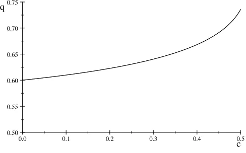
Share of …rms with aggressive accounting

For the high evasion regime, we get the following picture:

0.0 0.1 0.2 0.3 0.4 0.5

0.50 0.55 0.60 0.65 0.70 0.75

c q

Figure 5. The e¤ect of compatibility cost con

evasion share q, high evasion regime.

We plot the evasion share also for the values of compatibility costs beyond 0:2, that is when this equilibrium is not unique any more. The reason is that it is still a unique stable equilibrium (full cheating and full honesty are not stable). So from …gure 5 we can see that the e¤ect of the costs on the equilibrium share of evasion is positive, but quantitatively less pronounced than in the low evasion regime. An increase in costs from 0 to 0:25 leads to 5% increase (from 60% to 63%) in the share of …rms with aggressive accounting.

0.1 0.2 0.3 0.4 0.5 0.6 0.7 0.8 0.9 1.0 0.6

0.7 0.8 0.9 1.0

r q

Figure 6. The e¤ect of pro…t correlationr on

evasion shareq, high evasion regime,c= 0:1.

the e¤ect of the costs. An increase in correlation from 40% to 60% drives cheating down from around 64% to around 60%.

Auditing probabilities and tax revenues

The e¤ect of compatibility costs on auditing probabilities and tax revenues is summarized in the following table:

c q pHL _pLL _R

0 0:6 0:617 19 0:226 57 1:373 1 0:05 0:60465 0:618 24 0:232 54 1:362 5 0:1 0:60988 0:619 4 0:239 13 1:350 6 0:15 0:61582 0:620 7 0:246 46 1:337 0:2 0:62267 0:622 17 0:254 69 1:321 4 0:25 0:63071 0:623 85 0:264 08 1:303 0:3 0:64039 0:625 81 0:275 01 1:280 8 0:35 0:65244 0:628 18 0:288 06 1:253 1 0:4 0:6683 0:631 16 0:304 37 1:216 4

We see that both probabilities increase with an increase in compatibility costs. Again, the e¤ect is quantitatively small. An increase in costs from 0 to 0:25 leads to only 0.6 p.p. increase in the auditing probability for di¤erent reports and 3.8 p.p. increase in the auditing probability for similar reports. The tax revenues decrease, mirroring the case of low evasion.

Policy

The stylized examples above nicely illustrate di¤erent policies towards compat-ibility costs appropriate for di¤erent countries. The high evasion costs situation is more likely in developed countries with low level of evasion. In such cases the e¤orts to decrease compatibility costs can be dangerous in a sense of bringing about more cheating and lower tax revenues. The low evasion costs picture is for the countries with ‡ourishing evasion, like most of developing countries and CIS countries. These countries should not pay too much attention to compatibility of the accounts, as increasing the compatibility costs may result in even larger cheating.

5

Conclusion

The tax evasion game with costs of accounting compatibility between contracting …rms is considered in this paper. We show that when compatibility costs are small, there is a unique stable equilibrium10 _{with a positive share of evading …rms and a} positive share of audited reports. When the costs are large, there may be multiple equilibria, in some of which either everybody or nobody evades.

The game yields the insights that are impossible to obtain within the represen-tative …rm framework. Firstly, the tax authority should put more e¤ort in auditing …rms that did not coordinate their evasion decision, if it maximizes its expected rev-enue. Second, the compatibility costs may a¤ect the amount of evasion in the opposite directions depending on what the auditing technology and the equilibrium share of cheating are. If there are many non-compliant taxpayers, the compatibility costs are more likely to increase evasion, and visa versa. The correlation of taxpayer pro…t a¤ects equilibrium in a similar way. Third, the e¤ect of the …nes and auditing tech-nology on equilibrium values crucially depends on the prevailing accounting standard. When most of the …rms use an aggressive standard, an increase in …nes or auditing e¤ectiveness may have an adverse e¤ect on compliance.

There is a number of policy recommendations arising from our analysis. Firstly, compatibility costs reduction e¤orts are only justi…ed for economies (or industries) with substantial shadow sector. Such e¤orts include simpli…ed accounting (exogenous costs) and little interest in the business links (endogenous costs through auditing probability di¤erential). Secondly, the marginal increases in …nes may be dangerous in high evasion economies. Thirdly, compatibility costs enhancement may be a sensible strategy for low evasion countries, and it may even be …nanced by eventual reduction in enforcement costs.

We hope that our paper opens up a whole tile of issues that could not be addressed by the literature before. How do the links between taxpayers a¤ect their decision to pay taxes? How are these links taken into account by the tax authority? Could the government change the structure of these links for the bene…t of the whole society? We cannot answer these questions in a far too simpli…ed setting of business pairs we have here. However, what we can do is to say that the equilibrium behavior of the agents is a¤ected signi…cantly by the links between them, that it is a¤ected through the costs of behaving di¤erently, and it is a¤ected in the direction of harmonization

of this behavior.

References

[1] Alm, J. and M. Mckee (2004). Tax compliance as a coordination game. Journal of Economic Behavior & Organization 54, 297-312.

[2] Andreoni J., B. Erard and J. Feinstein. Tax Compliance. Journal of Economic Literature, June 1998, pp. 818-860.

[3] Bayer, R. and F. Cowell. Tax Compliance and Firms’ Strategic Interdependence.

Journal of Public Economics 93, pp 1131-1143 (2009) .

[4] Cowell, F. The Economics of Tax Evasion, MIT Press, 1990.

[5] Crocker, K. and J. Slemrod. Corporate Tax Evasion with Agency Costs.Journal of Public Economics, vol. 89(9-10), pages 1593-160, September 2005.

[6] Graetz M., J. Reinganum and L. Wilde. The Tax Compliance Game: Towards an Interactive Theory of Law Enforcement. Journal of Law, Economics and Or-ganization, 2(1), pp. 1-32, 1986.

[7] Lipatov, V. Social Interaction In Tax Evasion. MPRA Discussion Paper, 2008.

[8] Lipatov, V. Corporate Tax Evasion: the Case for Specialists. MPRA Discussion Paper, 2005.

[9] Reinganum J. and L. Wilde. Equilibrium Veri…cation and Reporting Policies in a Model of Tax Compliance. International Economic Review, 27(3), pp. 739-60, 1986.

[10] Sánchez-Villalba, M. (2006). Anti-evasion auditing policy in the presence of com-mon income shocks. Distributional Analysis Discussion Paper 80, STICERD, London School of Economics, London WC2A 2AE.

[11] Schneider, F. and Enste D. Shadow Economies: Size, Causes, and Consequences.

Journal of Economic Literature, pp.77-114, 2000

[13] Weibull, J. Evolutionary Game Theory. MIT Press, 1995.

Appendices

A - Proof of Lemma 1

The expected revenue of the auditor is

(1 q)2t + ( ) (1 q)t + q(1 q)t (22)

+ (1 +s)p aHL q(1 q)t (23)

( q(1 q) + ( ) (1 q))aHL

+ (1 +s)p aLL _q2_{+q( ) t}

q2+ 2q( ) + 1 2 + aLL

Here the …rst term is the revenue from the …rms that have high pro…ts and do not evade (they are of measure (1 q)2). The second group of 3 term is the revenue from the mixed reports: the high reports bringing t are of measure q(1 q) + ( ) (1 q), and low reports bringing in the …ne are q(1 q). Correspondingly, the costs of auditing must be subtracted for these cases. Finally, the last terms are the revenue from low reports and costs of auditing them. The same …ne is levied in the cases of two …rms or only one …rm misreporting.

Rearranging and taking …rst order conditions with respect to aLL _{and a}HL _gives

aHL : ( q(1 q) + ( ) (1 q)) + q(1 q) (1 +s)p0

aHL t = 0;

aLL : q2+q( ) (1 +s)t p0

aLL q2+ 2q( ) + 1 2 + = 0:

Working this out, we arrive at

gHL(q) : = q+

q(1 +s)t =p

0

aHL(q) ;

gLL(q) : = q

2_{+ 2q( ) + 1 2 +}

( q2_{+q( )) (1 +s)t} =p 0

aLL(q) ;

where the equality holds for a > 0. In this case we can show that p0

aHL_{(q) <} p0

aLL_{(q) , as}

gLL_{(q) g}HL_{(q) =} q2+ 2q( ) + 1 2 + q( q+ ) (1 +s)t

q+

q(1 +s)t

=

2

which is positive for any positive correlation and zero for independent draws. Note also that the di¤erence is decreasing and convex in q, so @2_p0

(a(q))=(@a@q) < 0,

@3_p0

(a(q))=(@a@q2_)>0.

Under concavity assumption second order conditions are trivially satis…ed and

aHL_{(q) > a}LL_{(q). Our intuition is con…rmed: low reports paired with high reports}

are audited more intensively than those paired with low reports.

Note though that because limq!0gHL(q) = +1, there may also be a corner

solution. Indeed, for any auditing function p(a) : lima!0p0(a) < +1 there will be

a corner solution. Formally, for all such functions 9q0

HL > 0 : aHL(q) = aLL(q) =

08q q0

HL. By construction it is also true that 9qLL0 > q0HL : aHL(q) > aLL(q) =

08q 2 [q0

HL; q0LL]. These threshold values can be found from the auditing function.

For the di¤erent reports we have

qHL0 =

= 1

p0_{(0) (1 +s)t 1}:

For the similar reports the threshold value f the share of …rms with aggressive ac-counting is implicitly de…ned by

1 2 + = (p0

(0) (1 +s)t 1) qLL0

2

+qLL0 ( ) ((1 +s)t 2):

Since 0 q0

HL 1, if p

0

(0) < 1=((1 +s)t ), tax authority will never audit, as the marginal revenue from audit is negative. Furthermore, ifp0

(0)< =( (1 +s)t ), the best response function is degenerate with a(q) 0; if p0

(0)<1 + 1=( (1 +s)t )

= , the similar reports are never audited: aLL_{(q) 0.}

Thus, both best responses (for mixed and similar reports) of the tax autority are weakly increasing continuous functions of q.

B - Proof of proposition 2

To show that p ; q is indeed a Bayesian Nash equilibrium, we need 1) p is a best response of tax authority given the belief aboutq; 2) each …rm plays best response to

p and the share of cheating …rmsq ; 3) the belief of the authority is consistent with equilibrium play of the …rms.

For 1) we need (??) and (1); for 2) in a mixed equilibrium it is su¢cient that each …rm is indi¤erent between cheating and honesty given that the partner is cheating with probability q:

or

(qu(L; L) + (1 q)u(L; H)) + ( )u(L; L) (1 q)c=

(qu(H; L) + (1 q)u(H; H)) + ( )u(H; L) qc

Rearranging, we get

(t b) (1 2q)c= ( (1 q))p aLL _{+ (1 q)p a}HL _{(1 +s)t : (24)}

Note that this expression depends on q unlike in the benchmark case, so we cannot present the resulting equilibrium explicitly. However, the two sides of the equation admit quite a straightforward intuitive explanation. The lhs is the bene…t from eva-sion net of accounting costsb and coordination costsc. The rhs is the expected cost of …nes in two types of matches: two low reports and high-low reports. Both costs and bene…ts of evasion increase with q. The higher population share of evaders relieves the coordination problem for a …rm that chose aggressive accounting. At the same time, higher share of wrong reports calls for more auditing thus increasing expected …ne.

Formally, from the properties of best response functionsaLL_{(q); a}HL_{(q)we can see}

that rhs of (24) is weakly monotonically increasing inq. Namely, it is zero forq q0

HL,

it is (1 q)p aHL_{(q) (1 +s)t for q 2 [q}0

HL; q0LL], and it is the full expression for q q0

LL converging to ( (1 q))p aLL (1 +s)t as q approaches unity. We

know thatp0

a(q)is convex (we can directly compute second derivatives). We also know

that p(p0

a)is decreasing, but we did not impose anything on its convexity/concavity.

Now,p(q)can be written asp(p0

a(q)). It is increasing, and it is also concave ifp(p

0

a)is

not too convex. Thus, rhs is concave under a mild ansumption on the third derivative of the function p(a).

Atq0

LL, the left derivative of rhs is (1 qLL0 )pq aHL(qLL0 ) p aHL(qLL0 ) (1 +s)t ,

the right derivative has an additional term ( (1 q0

LL))pq aLL(qLL0 ) + p aLL(qLL0 ) (1 +s)t ,

which is positive.

Lhs is linearly increasing in q with the slope2c, starting with (t b) c. The intersection(s) de…ne Bayesian Nash equilibrium. Because of a jump in the deriv-ative of rhs at q0

LL, we may have up to 6 intersections (with up to 3 locally stable

equilibria). However, the more interesting case for us is the stable unique equilib-rium, which indeed results for small values of c, if either (1 q0

LL)pq aHL(qLL0 ) p aHL_(q0

(1 +s)tmax_q2[q0

H L;q

0

LL] (1 q)p a

HL_{(q) . At the limit of no coordination costs,}

the equilibrium is de…ned by one of the conditions (1 b=t) = ( (1 q))p aLL _{+ (1 q)p a}HL

or (1 b=t) = (1 q)p aHL _{(1 +s), depending on the auditing technology. Namely,}

the …rst happens, if (t b) (1 2q0

LL)c > (1 qLL0 )p aHL(q0LL) (1 +s)t ,

and the second otherwise.

This equilibrium is unique and stable. By continuity, the same is true for small values ofc.

Note that with increase of c lhs simply rotates around horizontal line given by

(t b) . It retains this value atq = 0:5, while going down bycatq= 0 and up by

cat q= 1. This immediately leads us to the following corollary:

Corollary Withq= 1=2, the e¤ect of coordination costs is completely neutralized.

This is very intuitive: when the two populations are balanced, there is neither potential gain nor loss in terms of coordination from playing either strategy.

Note that the equilibrium will only be stable, if at the intersection the slope of the evasion costs (rhs) exceeds the slope of the bene…ts from evasion (lhs). Thus, stability requires the following condition to be satis…ed:

2c < (1 q )pq aHL_{(q ) p a}HL_{(q ) + ( (1 q ))pq a}LL_{(q ) + p a}LL_{(q ) (1 +s)t ;}

where q is the equilibrium share of the …rms that employ aggressive accounting. If there is no stable interior equilibrium, the full cheating is stable. A general condition for existence of full cheating equilibrium is u(A) u(C)givenq = 1. This can be rewritten, similarly to (24), as

(t b) +c p aLL_{(1) (1 +s)t ; (25)}

with p0

aLL_{(1) = 1=( (1 +s)t ).}

Full honesty may also be an option, if the auditing is cheap or payment for evasion high. A general condition for the existence of full honesty euilibrium isu(A) u(C)

given q= 0. This can be rewritten as

(t b) c 0:

However, this equilibrium is globally stable only if

C - comparative statics results

By inverse function theorem

aHL q = p

0 ₁ 0 q+

q(1 +s)t

0

q

=

q2_{(1 +s)t}

1

p00_(aHL₎; (27)

aLLq = p

0 ₁ 0 q2+ 2q( ) + 1 2 +

( q2_{+q( )) (1 +s)t} 0

q

= (28)

( q+ )2(1 +s)t + (2 q+ )

1 2 +

( q2_{+ ( )q)}2_{(1 +s)t}

1

p00_(aLL₎:

(29)

and

aHL k = p

0 1 0 q+

q(1 +s)t

0

q

=

q2_{(1 +s)t}

1

p00

(aHL₎; (30)

aLLq = p

0 ₁ 0 q

2_{+ 2q( ) + 1 2 +}

( q2_{+q( )) (1 +s)t} 0

q

= (31)

( q+ )2(1 +s)t + (2 q+ )

1 2 +

( q2_{+ ( )q)}2_{(1 +s)t}

1

p00_(aLL₎: