Modeling Internet Host Reliability using Higher-Order
Time Petri Net
Ali
M. Meligy
1Hani M. Ibrahim
2Amal M. Aqlan
3Professor of Computer Science Lecturer of Computer Science PhD candidate
1,2,3
Department of Mathematics, Faculty of Science, Menoufia University
ABSTRACT
The Higher-Order Petri Net is a new class of Petri Nets that exploit the properties of higher-order neural networks. Adding time to HOPN produces a new class called Higher-Order Time Petri Net, this is the subject of our study .In this paper, a method to model the internet host reliability with Higher-Order Time Petri Net is proposed. Analysis of HOTPN model is presented. A reachability graph is defined in a discrete way by using an enumeration procedure and the reachable states of the Time Petri Net and HOTPN. Finally, we compare between TPN and HOTPN by using the behavior properties and reachability graph.
Keywords:
Time Petri Net (TPN), Higher-Order Petri Net (HOPN), Reachability Graph, Internet Host Reliability.
1.
INTRODUCTION
Petri nets have many applications in different issues in the different systems. These systems may be complex. It is for this reason that different Petri net types have been formally defined and created. Every one of them has its own particular specialized use which is very interesting to solve and address a particular problem. But having so many different types of Petri nets creates issues as how to choose the best Petri net type or class for a particular problem. Petri nets can be used to test and verify rigorously, system functionality and design implications at the very initial phases of analysis. They can be used to determine critical performance issues related to time and failure. Petri nets can be used to create different viewpoints of a system related to the conceptual, logical or physical design structures [1].
In some cases, the classical Petri nets cannot model the behavior of the system accurately. To solve this problem, researchers proposed a new class of Petri nets called Higher Order Petri Nets (HOPN) that are based on the properties of higher-order neural networks.
Time Petri Nets are derived from classical Petri nets. Additionally, each transition t is associated with a time interval [at, bt]. Here, at and bt are relative to the time, when t was enabled last [2]. Every possible situation in a given TPN can be described completely by a state z = (m, h), consisting of a (place-) marking m and a transition marking h.
A reachability graph RG(Z) for a TPN Z can be defined in such a way that its vertices are the reachable integer-states or the reachable essential-states, respectively. The edges are defined by the triples (z, t, zʹ) and (z, τ, zʹ), τ ∈ N, where zt z and
z
z , respectively. This graph is finite if and only if the set of the reachable markings of the net is finite. An enumeration procedure for computing the reachable graph of a given TPN can be constructed easily.
The most important behavioral properties of a TPN (and of a PN as well) are the reachability, the boundedness and the
liveness. These properties are decidable for an arbitrary classical PN, but not for an arbitrary TPN in general. However, there are restricted classes of TPN for which the properties are decidable.
In paper [3] used method to model the internet host reliability with Time Petri nets While in this paper we will discuss modeling the internet host reliability with HOTPN.
This paper is organized as follows. The next section introduces some preliminary definitions and remarks. Next section, discusses definitions proposed of Higher-Order Time Petri Net, represents reachability graph, analyze of HOTPN and Comparison between two models (TPN and HOTPN) by behavior properties.
2.
BASIC NOTATIONS AND
DEFINITIONS
Definition 1 (Higher-Order Petri Net) An HOPN is formally defined in the same way as the classical Petri nets, HOPN = (P, T, F, W, M0), where [4]
F ⊆ (P×T) ∩ (P2×T) ∩………. ∩ (Pm×T) ∩ (T×P) is a set of arcs.
W: F → Ν is a weight function;
M0: P → Ν is the initial token distribution, called the initial marking.
The main difference is the definition of the set of arcs.
Definition 2 (Firing Rule of HOPN) A transition t is said to be enabled or firable if there exist at least one of its kth-order input arcs such that each of this arc’s places have at least as many tokens as the weight of this kth-order arc. Such an arc is defined as an enabled arc.
Definition 3 (Time Petri Net) The structure Z = (P, T, F, V, M0, I) is called a Time Petri net (TPN), if [2]
S(Z) := (P, T, F, V, M0) is a Petri nets, i.e. P, T, F are finite sets with P ∩ T = φ, P ∪ T ≠ φ, F ⊆ (P × T ) ∪ (T × P), V : F → N+ (weight of the arcs), M0 : P → N (initial marking).
: ( { })
0
0
Q Q T
I and I1(t) ≤ I2(t) for
each t ∈ T , where I(t) = (I1(t), I2(t)).
The Petri net S(Z) is referred to as the skeleton of Z. I is the interval function of Z, I1(t) and I2(t) are the earliest firing time of t (eft(t)) and the latest firing time of t (lft(t)), respectively. A transition t is called immediate, if eft(t) = lft(t) = 0. A TPN is called strong, if there does not exist an infinite latest firing time in the net, i.e.,
0 0
:T Q Q
I . In a strong TPN, each transition is forced to fire within a finite time interval.
Definition 4 (state) Let Z = (P, T, F, V, M0, I) be a TPN and
} # {
: 0
R T
25 M is a reachable marking in S(Z),
∀t ((t ∈ T ∧ t− ≤ m) → h(t) ≤ lft(t)) and ∀t ((t ∈ T ∧ t− ≮ m) → h(t) = #).
The state z0:= (m0, h0) with is set as the
initial state of the TPN Z.
The interpretation of the notion “state” is as follows: within the net, each transition t has a clock h(t). If t is enabled at a marking M, its clock h(t) shows the time elapsed since t became most recently enabled. If t is disabled at m, the clock is switched off (indicated by h(t) = #). Thus, the vector h which is a vector of clocks is actually a transition marking and the already defined notion “marking” is in fact a place marking. In the following we call the places marking M a p-marking and the transitions marking h a t-marking. The state z = (m, h) is called an integer state, if h(t) is an integer for each enabled transition t in m. Each transition t T induces the marking t− and t+, defined as follows:
F p t iff
F p t iff p t W t F t p iff
F t p iff t p W t
) , ( 0
) , ( ) , ( ,
) , ( 0
) , ( ) , (
and t−≤ m (i.e. t−(p) ≤ m(p) for every place p P).
The behavior of a TPN is defined by changing from one state into another by firing a transition or by time elapsing.
Definition 5 (state changing) Let Z = (P, T, F, V, M0, I) be a TPN, tˆ be a transition in T and z = (m, h), z0 = (m0, h0) be two states [2]. Then
the transition is ready to fire in the state z = (m, h), denoted by ztˆ , iff
i.
t
ˆ
m
and ii. eft(tˆ) ≤ h(tˆ). the state z = (m, h) is changed into the state zʹ = (mʹ, hʹ)
by firing the transition tˆ, denoted by
z
tˆz
, iff i. tˆ is ready to fire in the state z = (m, h) ii.m
m
t
ˆ
andiii.
otherwise t t m t m t iff t h
m t t
h T t t
0
ˆ )
(
iff # )
(
(
Where
t{p|pP(p,t)Fandˆtdenotes tˆ tˆ
the state z = (m, h) is changed into the state zʹ = (mʹ, hʹ) by the time elapsing
0 R
, denoted byz
z
, iffi. mʹ = m and
ii.
t
(
t
T
h
(
t
)
#
h(t)
lft(t)
(i.e. the time elapsing τ is possible), andiii.
m m t iff t h t h T t
t
-t iff #
) ( ) (
(
Definition 6 (Reachability Graph) The graph RGz(z0) is called a reachability graph of the time Petri net Z iff its nodes are the integer-states from Zz(z0) and its arcs are defined by the triples (z, τ, zʹ) and (z, t, zʹ), where z zandzt z, respectively [5].
Definition 7 (Boundedness) Let Z = (P, T, F, V, M0, I) be a TPN.
A place p P is called bounded (at z0) iff there exists a natural number K with m(p) ≤ K for each marking m Rz(z0),
The net Z is bounded (at z0) iff all places p are bounded (at z0).
Definition 8 (Liveness) Let Z = (P, T, F, V, M0, I) be a TPN, z a reachable state and t T [2].
t is called live in the state z iff:
)) )
( ( ) (
(
t
z z z z z RS z z RS
z
z (i.e. t is ready to
fire inz)
Z is live iff all transitions are live in z0.
The set of all reachable states in Z, starting at
z
z
0,is denoted byRS
z(
z
)
.Definition 9 (Reachability) Let Z = (P, T, F, V, M0, I) be a TPN,
The state z = (m, h) is called reachable in Z (starting at z0), if there exist states z1, z1ʹ, ..., zn, znʹ, transitions t1, ..., tn and times τi∈ R0, i = 0, 1, ..., n and it holds
z
z
z
z
z
z
z
z
n nn t n t
t
0 1 1 2 2
2 2 1 1 0
The sequence of transitions σ = t1 . . . tn can fire in Z starting at z0, because there is a sequence ()0t11tnn. We call such a transition sequence σ a feasible one (or a firing sequence for short). The sequence σ(τ), which is a concrete execution of σ in Z, is called a (feasible) run of σ. It is clear that in a given TPN the state changes generally consist of alternating series of time elapsing and transition fires. Obviously, for a given run the transition sequence is well defined, and for a given transition sequence there are infinitely many runs in general.
Definition 10 (An Enumeration Procedure of TPN) Starting at the initial state all state successors of a reached integer-state can be derived in a successive way (i.e. breadth-first search) [6]:
Basis: z0 RG(Z),
Step: Let z be in RG(Z) already. 1. For i=1 to n do
If
z
t1z
possible in Z (cf. def 5) then z′ RG(Z)end
2. If
z
t1z
possible in Z (cf. def 5) then z′ RG(Z)3.
THE PROPOSED HIGHER-ORDER
TIME PETRI NET
We now integrate the concept of the network with the concepts of Net to obtain new definitions and suitable for the proposed class.
0 0 0
# 0 ) (
m t iff
3.1
The Proposed Definitions of HOTPN
Definition 11 (Higher-Order Time Petri Net) The structure HOZ = (P, T, F, V, M0, I) is called a Higher-Order Time Petri net (HOTPN), if
S(HOZ) := (P, T, F, V, M0) is a Higher-Order Petri nets,
: ( { })
0
0
Q Q T
I and I1(t) ≤ I2(t) for
each t ∈ T , where I(t) = (I1(t), I2(t)).
Definition 12 (Firing rule of HOTPN) A transition t is said to be enabled or firable if
There exist at least one of its kth-order input arcs such that each of this arc’s places have at least as many tokens as the weight of this kth-order arc.
the state z = (m, h) is changed into the state zʹ = (mʹ, hʹ)
by firing the transition tˆ, denoted by
z
tˆz
, iffi. tˆis ready to fire in the state z = (m, h) ii.
m
m
t
ˆ
andiii.
otherwise t t m t m t iff t h
m t t
h T t t
0
ˆ )
(
iff # )
(
(
Definition 13 (Reachability Graph) The graph RGHOz(z0) is called a reachability graph of the Higher-Order Time Petri net HOZ iff its nodes are the states from HOZz(z0) and its arcs are defined by the triples (z, τ, zʹ) resp. (z, t, zʹ), where
z z resp z
z . t .
Definition 14 (Boundedness) Let HOZ = (P, T, F, V, M0, I) be a HOTPN.
A place p P is called bounded (at z0) iff there exists a natural number K with m(p) ≤ K for each marking m Rz(z0),
The net HOZ is bounded (at z0) iff all places p are bounded (at z0).
Definition 15 (Liveness) Let HOZ = (P, T, F, V, M0, I) be a HOTPN, z a reachable state and t T
t is called live in the state z iff:
)) )
( ( ) (
(
t
z z z z z RS z z RS
z
z (i.e. t is ready to
fire in z)
HOZ is live iff all transitions are live in z0.
Definition 16 (Reachability) Let HOZ = (P, T, F, V, M0, I) be a HOTPN,
The state z = (m, h) is called reachable in HOZ (starting at z0), if there exist states z1, z1ʹ, ..., zn, znʹ, transitions t1, ..., tn and times τi∈ R0, i = 0, 1, ..., n and it holds
z
z
z
z
z
z
z
z
n nn t n t
t
0 1 1 2 2
2 2 1 1 0
3.3
The Modeling of HOTPN
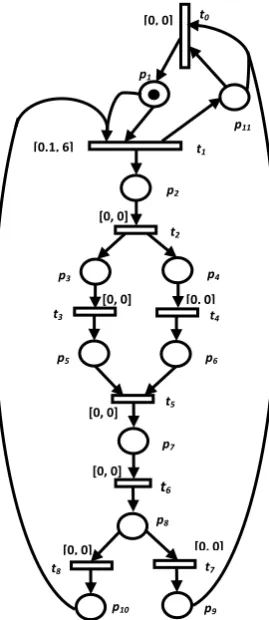
In this section, we build a model for internet host reliability using Higher-Order Time Petri net from Time Petri Net. In Fig.2 (cf. [3]) is a extension of Fig.1 by the introduction of second-order arc of transition t1. We note the most important differences between the two figures, as follows
The static behaviour of model can be represented using
places, transition and arcs.
a. An increase in the number of places (p11), then become the number 11 instead of 10.
b. The same number of transitions.
c. The emergence of a second-order arc of p1 and p10 to t1. Also the emergence of a second-order from p9 and p11 to t0.
The dynamic behaviour of model can be represented using token inthe state of the model.
a. The number of token in initial state is 10
1 0(1,0,0,0,0,0,0,0,0,0)
M in TPN. While in
HOTPN is
11 1 0(1,0,0,0,0,0,0,0,0,0,0)
M
.
In Fig. 1, we note the presence of a single period of time on the transition t1, while the rest transitions (t2 to t9 and t0) do not contain the times. Thus, we suppose that part of the net that contains places p1, p2, p10 and p11 and transition t1) is a subnet which denoted HOZ1. While denote to the other part HOZ2. In the subnet HOZ1, in the initial state, the transition t1 is enabled, thus, z0 can change into another state only as time elapses. For example, the change of
i i
z
z 1
* 1 . 0
0 is feasible,
where z1 is given by
1 9 11 1 1
1 1
# # i * 0.1
#
, 0 0 0 1 ) , (
i i
i m h
z
and m1i m0, i1,2,,60, 0 0.1*i In z1i the transition t1 can fire, yielding state z2 where
1 9 11 1 2
2 2
# 0 # #
, ) 0 0 1 0 ( ) , (
h m z
Thus, the sequence
2 1 * 1 . 0 0
1 z
z
z i t
i
is executable in HOZ1. It present in every sequences firing in net HOZ.
3.3
Analysis of HOTPN
To analyze the behavior of Model using the reachability graph and it apply behavioral properties.
3.3.1
The Sequences of Transitions:
a. The state space of Time Petri net (Z) is the set of all reachable states of the net is (σ1, σ2, σ3, σ4), where
}, , , , , , , ,
{1 2 3 4 5 6 8 0 1 t t t t t t t t
}, , , , , , , ,
{1 2 4 3 5 6 8 0 2 t t t t t t t t
27 Fig. 1: Modeling Internet Host Reliability using HOTPN.
} , , , , , ,
{1 2 3 4 5 6 7 3 t t t t t t t
, } , , , , , ,{1 2 4 3 5 6 7 4 t t t t t t t
More detail 2 0 8 6 5 4 3 2 1 1 0 9 7 6 5 3 2 2 1 * 1 . 0 0 1()Z t t t t t t t Z t i i M M M M M M M z z z t 2 0 8 6 5 3 4 2 1 1 0 9 7 6 5 4 2 2 1 * 1 . 0 0
2()
Z t t t t t t t Z t i i M M M M M M M z z z t 2 7 6 5 4 3 2 1 1 8 7 6 5 3 2 2 1 * 1 . 0 0
3()
Z t t t t t t Z t i i M M M M M M z z z t 2 7 6 5 3 4 2 1 1 8 7 6 5 4 2 2 1 * 1 . 0 0
4()
Z t t t t t t Z t i i M M M M M M z z z t
b. The state space of an Higher-Order Time Petri net (HOTPN) is the set of all reachable states of the net is (σ1, σ2, σ3, σ4), where
}, , , , , , , , ,
{1 2 3 4 5 6 8 0 1 1 t t t t t t t t t
}, , , , , , , , ,{1 2 4 3 5 6 8 0 1 2 t t t t t t t t t
} , , , , , , ,{1 2 3 4 5 6 7 0 3 t t t t t t t t
, } , , , , , , ,{1 2 4 3 5 6 7 0 4 t t t t t t t t
More detail 2 1 0 8 6 5 4 3 2 1 1 1 10 9 7 6 5 3 2 2 1 * 1 . 0 0 1()HOZ t t t t t t t t HOZ t i i M M M M M M M M z z z t 2 1 0 8 6 5 3 4 2 1 1 1 10 9 7 6 5 4 2 2 1 * 1 . 0 0
2()
HOZ t t t t t t t t HOZ t i i M M M M M M M M z z z t 2 0 7 6 5 4 3 2 1 1 0 8 7 6 5 3 2 2 1 * 1 . 0 0
3()
HOZ t t t t t t t HOZ t i i M M M M M M M z z z t 2 7 6 5 3 4 2 1 1 0 8 7 6 5 4 2 2 1 * 1 . 0 0
4()
HOZ t t t t t t t HOZ t i i M M M M M M M z z z t o
The enumeration procedure for computing the reachable graph of a given TPN defined above can be performed using the definition 5. The reachability graph of the TPN is shown in Fig.2.
3.3.2
The behaviour properties of the models
Depending on definitions of TPN (and HOTPN) properties and Fig. 2 (and Fig.3), we can deduce following table.
Table 1: comparison of the behavioral properties between the TPN and HOTPN
properties TPN model HOTPN model
Boundedness All sequences All sequences
Liveness
1 and 2 are live, 3 and 4 are not live
All sequences
reachability All sequences All sequences
[image:4.595.102.237.82.393.2]t8 t4 p11 [0, 0] [0, 0] p8 t7 p9 p10 [0, 0] [0, 0] t6 t5 p7 [0, 0] [0.1, 6] [0, 0] [0, 0] [0, 0] t0 t3 t2 t1 p6 p5
p3 p4
p2
Fig. 2: The reachability graph of the TPN model in ref. [3].
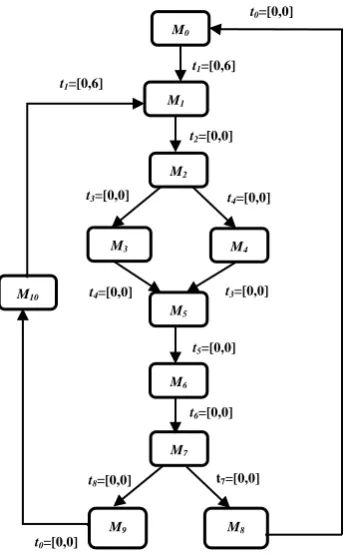
Fig. 3: The reachability graph of the HOTPN model in Fig.1
From Table 1 we note that:
TPN model is reachability, Boundedness and not liveness.
HOTPN model is reachability, Boundedness and liveness.
Table 4 summarizes the place set of the reachability graph. The header represents places and the left-most column represents the place set having marking. The reachability analysis was very useful to validate state transitions of the places.
Table 2: Place set of the reachability graph of the HOTPN model in Fig. 3
P1 P2 P3 P4 P5 P6 P7 P8 P9 P10 P11
M0 1 0 0 0 0 0 0 0 0 0 0
M1 0 1 0 0 0 0 0 0 0 0 1
M2 0 0 1 1 0 0 0 0 0 0 1
M3 0 0 0 1 1 0 0 0 0 0 1
M4 0 0 1 0 0 1 0 0 0 0 1
M5 0 0 0 0 1 1 0 0 0 0 1
M6 0 0 0 0 0 0 1 0 0 0 1
M7 0 0 0 0 0 0 0 1 0 0 1
M8 0 0 0 0 0 0 0 0 1 0 1
M9 0 0 0 0 0 0 0 0 0 1 1
M10 1 0 0 0 0 0 0 0 0 1 0
4.
CONCLUSIONS
This paper discusses internet host reliability modeling using Higher-Order Time Petri Net. Thus, an enumeration procedure can compute a reachability graph for a given HOTPN. The behaviour of the net can be studied by graph and properties. Thus, the HOTPN solves live problem in TPN model. Therefore, the HOTPN is live when its skeleton is live.
5.
REFERENCES
[1] Staines, A., 2010 Supporting Requirements Engineering with Different Petri Net Classes" International journal of computers, vol.4 (4).
[2] Bachmann, J. and Popova-Zeugmann, L., 2010 Time-independent Liveness in Time Petri Nets. IOS Press, Fundamental Informaticaevo, vol.101, pp.1–17.
[3] Meligy, A., Ibrahim, H., and Aqlan, A., 2012 Internet Host Reliability Modeling with Time Petri Nets. International Journal of Computer Applications, vol.47, no.16.
[4] Chow, T., Li, J-Y. , 1997 Higher-Order Petri Net Models Based on Artificial Neural Networks. Artificial Intelligence, V. 92, pp. 289-300.
[5] Popova, L., 1991 On Time Petri Nets. J. Inform. Process. Cybern. EIK 27(1991)4, pp. 227–244.
[6] Popova-Zeugmann, L., 2007 Time Petri Nets State Space Reduction Using Dynamic Programming. Journal of Control and Cybernetics, 35(3):721–748.
t0=[0,0]
t1=[0,6]
t2=[0,0]
t4=[0,0]
t3=[0,0]
t3=[0,0]
t4=[0,0]
t5=[0,0]
t8=[0,0]
t6=[0,0]
t7=[0,0]
M0
M2
M1
M3 M4
M5
M8
M6
M7
M9
t1=[0,6]
t0=[0,0]
t0=[0,0]
t1=[0,6]
t2=[0,0]
t4=[0,0]
t3=[0,0]
t3=[0,0]
t4=[0,0]
t5=[0,0]
t8=[0,0]
t6=[0,0]
t7=[0,0]
M0
M2
M1
M3 M4
M5
M8
M9
M6
M7