Audio Compression using Multiple Transformation
Techniques
Rafeeq Mohammad
M-Tech Student, Dept of ECE Gudlavalleru Engineering CollegeGudlavalleru (A.P), India
M. Vijaya Kumar
Asst. Professor, Dept of ECE Gudlavalleru Engineering CollegeGudlavalleru (A.P), India
ABSTRACT
The paper presents a comparative study of audio compression using multiple transformation techniques. Audio compression with different transform techniques like Discrete Cosine Transform, Wavelet Transform, Wavelet Packet Transform (W.P.T) & Cosine Packet Transform is analyzed and compression ratio for each of the transformation techniques is obtained. Mean Compression ratio is calculated for all of the techniques and compared. Performance measures like signal to noise ratio (SNR), normalized root mean square error (NRMSE), retained signal energy (RSE) are also calculated and compared for each transform technique. Transform based compressed signals are encoded with encoding techniques like Run-length Encoding (R.L.E) and Mu-Law Encoding to reduce the redundancies. From the comparison it is clear that Discrete wavelet transform gives better compression ratio of about 27.8593 compared with the other three transforms. Mean SNR value is minimum for DCT 29.2830, and comparatively higher mean SNR value 43.4037 for CPT.
General Terms
Audio data compression
Keywords
CPT, WPT, NRMSE, RSE, RLE
1.
INTRODUCTION
Audio is an electrical representation of sound. In general audio is sound within the range of human hearing. Specifically it ranges from 20 Hz to 20 kHz. This range of frequency is detectable by the human ear. The concept of Audio Compression is to compress the audio data so that it occupies less space for storing data. The need for audio compression is to accommodate more data in the available storage area so that the storage capacity can be enhanced [16]. Due to occupancy of less storage space, more amounts of data can be placed in the available memory, (efficient use of memory).
As a result of less storage space for data occupancy, more amount of data can be transmitted with less transmission bandwidth. That means compressed audio signal can be transmitted over the internet with less transmission bandwidth and higher speeds. As a result of increased speed, audio files can be uploaded and downloaded over the internet faster with higher bit rates. Due to fast downloading and uploading of audio files time delay is minimized.
Like general Data compression, Audio compression is also classified in to two categories.
i) Lossy Compression ii) Loss-less Compression
Lossy compression is a data encoding method that compresses data by losing some part of data that is discarding data. Lossy compression is most commonly used to compress multimedia data like audio signals, especially in applications like streaming media and internet telephony. In this paper, lossy audio compression method like Mu Law Encoding technique is carried out. The advantage of lossy compression over lossless compression is that in certain cases a lossy method produces much smaller compressed file than lossless method and still reaches the requirements of the application. Mu-law encoding technique is lossy compression technique. By using lossy compression technique file size can be minimized by losing some information of the original data [21].
Lossless data compression is a technique that decompresses data back to its original form without any loss. In this compression technique the decompressed file and original file are identical, that is original data reconstructed from the compressed data. Run length encoding technique, implemented in this paper is a lossless compression technique. Lossless compression techniques have been used to compress audio signals, by finding redundancies and removing it. Lossless techniques such as Run-length encoding can be applied directly to the audio files for audio compression for significant compression. Audio signal is compressed by removing redundancy between adjacent samples.
Fig.1 Overall Block Diagram
The overall block diagram of the audio compression process is shown in Fig.1. While applying wavelets and packet based transforms (like wavelet packets and cosine packets) the first step is sub-band decomposition or packet decomposition then the respective transform or filter coefficients will be applied on decomposed elements. A threshold is applied to coefficients to each level from 1to N. Several wavelet coefficients are zero or near to zero. By applying thresholding near to zero coefficients values are equal to zero [1],[2]. As the coefficient below the threshold level is zero, many consecutive zeros produced can be stored in much less space and transmission speed will be increased. In the final stage, the compressed audio is encoded with encoding techniques.
2.
TRANSFORM TECHNIQUES
2.1
Discrete cosine transform
Discrete cosine transform, linearly transforms data into frequency domain, so that the data can be represented by a set of coefficients. The benefit of discrete cosine transform is that, the energy of the actual data may be concentrated in only a few low frequency components of DCT depending on the correlation present in the data. Equation (1) represents the D.C.T of 1-dimentional sequence of length N.
And for u = 0, 1, 2… N−1. Similarly, (2) represents the inverse transformation (IDCT).
Likely for x= 0, 1, 2 …N− 1. In both equations (1) and (2) α (u) is defined as
α (µ) = √1/N for u=0
and
α (µ) = √2/N for u≠0
Wavelet: Wavelet is a part of waveform, whose average energy value approximately tends to zero. Generally, wavelet is a varying window length considered as a part of waveform. Wavelet transform are based on small wavelets with limited duration.
Equation (3) and (4) shows mathematical representation of wavelet [5]. ѱ(t) is a function called mother wavelet.
2.2
Discrete wavelet transform
Jean Morlet introduced the idea of wavelet transform in 1982 and provided mathematical tool for seismic wave analysis [5]. In equation (5) Morlet considered wavelets as a family with functions constructed from translations of single function called ‘mother wavelet’ ѱ(t). It is given in(5) where a, b ∈ R and a ≠ 0.
The parameter ‘a’ is the scaling parameter and it measures the degree of compression. And parameter ‘b’ is translation parameter and it determines the time location of the wavelet [5]. DWT decompose signal in to several n levels in different frequency bands. At each step there are two outputs, scaling and wavelet coefficients. The equations (6) and (7) represent the scaling and wavelet coefficients respectively.
Wavelet transforms convert a signal in to series of wavelets and they provide a way for analyzing waveforms in both frequency and time duration. Wavelet transforms are a mathematical means to perform signal analysis when signal frequency varies with time [14], [15]. The Wavelet transform provides the time-frequency representation. That is, wavelet transforms provide time and frequency information at the same time, hence giving a time-frequency representation of the signal [5].
2.3
Wavelet packet transform
Wavelet packets, (which is known as Wavelet packet decomposition) is a wavelet transform where the discrete-time sampled signal is passed through more filters than the Discrete Wavelet transform. Wavelet packets are the particular linear combination of wavelets. Wavelets provide bases which retain many properties like i) orthogonality ii) smoothness and iii) localization of the parent wavelets. The coefficients in linear combination are computed by a repetitive (recursive) algorithm making each newly computed wavelet packet coefficient sequence the root of its own analysis tree [6],[9][10].
d
m,j= [
d
m,j]
∈
R
Nd
Wavelet coefficient vectors in equation (8) represent uniformly distributed frequency banks, where Ndis number
of wavelet coefficients in the coefficient vector dmj [6]. Decomposition scheme may be represented by a full binary tree [11],[12].
Packet De-composition
Transform Technique
Extract Coefficients
Threshold Detector Compressed
Audio Encoding
(RLE, Mu law)
I/P
Wwpt = {Wm,j wpt}m,j :Wm,j wpt ↔ dm,j (9)
With sample frame of audio signal ‘d00’ related to its root and wavelet coefficientsdm,j related to its nodes and leafs, the best wavelet basis sub tree is given by (10).
The advantage of wavelet packet decomposition is that it is possible to select the optimum binary tree to analyze for a given signal. The choice of optimization depends on the application, where the decomposition is to be applied. The wavelet packet transform have several applications. And one of the application is calculation of the best basis [3] , [4].
Wopt = *
arg min
W *
mj mj
x W
x
(10)2.4
Cosine packet transform
The cosine packet Transform is a scheme, that allows time splitting decomposition prior to the frequency transformation [13]. If we consider that, the original signal in the time domain being spited successively in to two halves, a tree configuration will be resulted at each iteration. If the transform imposes no restriction on the support intervals of the window, then it is not needed to be combined in the same way the subspaces do not need to be of equal size. So in analogy to the wavelet packet case, one is now faced with large number of possible orthonormal basis configurations, each one of them being considered as a cosine packet [8],[17]. It is important to observe that in the cosine packet case, the windows do not need to be of a dyadic size, they may be an arbitrary size. Equation (11) represents the family of local cosine basis function and it can be written as
Where the function bk is a smooth window [8]. Equation (12) defines local cosine functions and it is represented as
Where Ck,n (x) is the family of basis functions of DCT. However, in this paper, only dyadic sized windows are considered. We note that, as one goes down the tree, time resolution is improved by a factor of two at each layer, while frequency resolution is reduced by a factor of two, at each iteration. Cosine packets are generalizations of discrete cosine transform [8].
3.
ADAPTIVE THRESHOLD
3.1
Threshold Detector
One of the most important process in the compression algorithm is threshold detection. The role of this is to nullify all the coefficients obtained from the transforms to a smaller threshold value [13]. Assuming that the distortion parameter of compression system as ‘a’, N as number of samples of signal to be processed and Ex as the energy of the input audio signal, then the equation (13) represents threshold value.
Constant ‘a’ can be related with the SNR of input signal and
is given in (14)
The parameter ‘a’ in (14) is represented by (15) as
Where an is lower bound of ‘a’. Using (13) and (15) lower bound value for the threshold is given in (16).
4.
ENCODING TECHNIQUES
4.1
Run length Encoding:
Fig.2 Run Length Encoding Flow Chart
Two encoding methods are implemented, in order to encode transformed coefficients obtained after applying transforms. Run-length encoding is a popular data compression algorithm in which Runs of data (that is, sequences in which same data values occur in many consecutive data elements) are stored as a single data value and count, rather storing original repeated runs. This type of encoding (RLE) is very useful in data which contain many repeated runs. Run length encoding is lossless data compression technique in which runs of data is stored as
Count of Run = 0
Read Run value X
Read Run value Y
RunX== RunY
String ends?
Write Run Count value
Write the Run value X
Run value of X = = Run value of Y
Run Count =0 Write Run count
vaue
Run value X= 0
Count is Max?
No
Yes
Exit
Increment Run count
No
single data value and followed by count [2]. RLE works by reducing the physical size of a repeating string of characters. This repeating string, called a ‘run’, is typically encoded into two bytes. The first byte represents the number of characters in the run and is called the ‘run count’. The second byte is the value of the character in the run, which is in the range of 0 to 255, and is called the ‘run value’.
The flow chart shown in figure.(2) shows the basic flow during the run length encoding. First the Run Count is initiated to zero, after that count reads the run values viz. Run A, Run B and so on. . If it is end of data stream then it writes the first run value. If run count value is not end of data stream then it checks whether run count value of A equal to run count B. If equal, again checked whether run count is maximum then count is incremented. If the count not equal then it writes run count value A and checks whether it is equal with the run count value B, if equal then Run count made zero and the process continues again.
4.2
Mu- Law Encoding
Mu-law is audio compression scheme that compress 16 bit linear data down to 8 bits of logarithmic data [7],[19]. The encoding process breaks the linear data into segments with each progressively higher segment size is doubled. This ensures that the lower amplitude signals get the highest bit resolution while still allowing enough dynamic range to encode high amplitude signals. This method provide a compression ratio of about 2:1. But Mu- Law encoding does not require much processing power to decode. Mu-law is a standard companding format specified in CCITT G.711 recommendation [7]. Mu-law mostly used in digital communications systems in North America and Japan. The Mu-Law Compressor block implements a µ-law compression using (17) for the input signal. The formula for the µ-law compressor is given by (17)
y={ [ V log (1+µ|x |/V) ]÷[ log(1+µ) ] }* sgn (x) (17)
Where µ is the µ-law parameter of the compressor, V is the peak magnitude of x, log is the natural logarithm, and sgn is the signum function in (17).
5.
PERFORMANCE MEASURES
For the audio compression method, based on transform techniques, the performance is measured in terms of Compression ratio, SNR, NMRSE, RSE.
Compression ratio
: Compression ratio (C.R) is defined as ratio between Length of original signal and Length of compressed sigal.
[image:4.595.322.536.72.418.2]
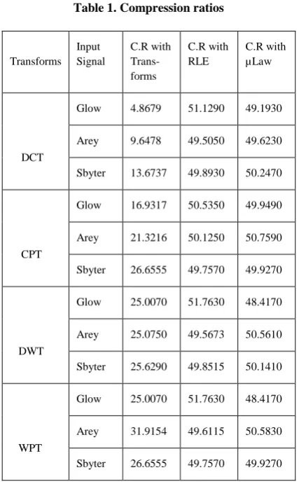
The compression ratios for different audio signals after applying each transform technique and compression ratios after applying the encoding techniques (Run- Length Encoding and Mu- Law Encoding) are tabulated in Table-1.The performance measures like signal to noise ratio, normalised root mean square error, and retained signal energy are measured. The mathemetical representations of these performance parameters or measures (viz. SNR, NRMSE, RSE) are represented in equations (19),(20) and (21).
Table 1. Compression ratios
Transforms Input Signal
C.R with Trans-forms
C.R with RLE
C.R with µLaw
DCT
Glow 4.8679 51.1290 49.1930
Arey 9.6478 49.5050 49.6230
Sbyter 13.6737 49.8930 50.2470
CPT
Glow 16.9317 50.5350 49.9490
Arey 21.3216 50.1250 50.7590
Sbyter 26.6555 49.7570 49.9270
DWT
Glow 25.0070 51.7630 48.4170
Arey 25.0750 49.5673 50.5610
Sbyter 25.6290 49.8515 50.1410
WPT
Glow 25.0070 51.7630 48.4170
Arey 31.9154 49.6115 50.5830
Sbyter 26.6555 49.7570 49.9270
.
Signal to noise ratio
: Signal to noise ratio is a measure
that compare the level of desired signal to the level of background noise.
σs2
the mean square of audio signal and σe 2
is mean square difference between original and reconstructed audio signal.
Normalised root mean square error:
x(n) is the audio signal, x'(n) is reconstructed or compressed audio signal. Generally RMSE represents the standard deviation of the differences between predicted values and observed values.
Retained Signal Energy:
Table 2. Performance Parameters
Transforms Input Signal
SNR NRMSE RSE
DCT
Glow 58.4953 0.3054 0.0661
Aray 17.2306 0.3131 0.0510
Sbyter 12.1232 0.3140 0.0180
CPT
Glow 43.4551 0.3090 0.0669
Aray 43.4100 0.3122 0.0508
Sbyter 43.4391 0.3164 0.0181
DWT
Glow 28.9873 3.5466 0.0034
Aray 37.6697 1.3070 0.0040
Sbyter 51.2340 0.2743 0.0050
WPT
Glow 28.9873 3.5466 0.0034
Aray 55.3519 3.0334 2.2085
Sbyter 43.3491 0.3164 0.0181
The performance parameter values like signal to noise ratio, normalized root mean square error, and retained signal energy are measured using the formulae (19) (20) and (21).
And the corresponding performance measure values, that is measured performance parameters like SNR, NRMSE and RSE are tabulated in the Table 2.
Mean compression ratio is the average of the compression ratios. Mean compression ratios are calculated for each of the four transform techniques using different audio samples.
Mean values are calculated for both the transform based compression and encoding based compression techniques. Similarly, mean SNR values are calculated for different transform techniques and audio signals. The values of mean compression and mean SNR are tabulated in the Table 3.
[image:5.595.55.282.93.400.2]Normalised root mean square error and retained signal energy values are also tabulated in the performance parameters table.
Table 3 Mean Compression ratios
Trans-forms
C.R with Trans-forms
C.R with RLE
C.R with Mu-law
Mean SNR
DCT 9.3964 50.1756 49.6876 29.2830
CPT 21.6362 50.1390 50.2116 43.4047
DWT 25.2370 50.3939 49.7063 39.2970
WPT 27.8593 50.3771 49.6423 42.5627
6.
RESULTS
Several audio signal samples are simulated using MATLAB. DCT is computed using the equation (1). Transform coefficients are extracted for further processing. Compression is obtained with transform techniques, adaptive thresholding and encoding techniques like run length and mu law encoding techniques. Energy of the input signal is computed and threshold value is calculated with equation (16). The value of input energy is compared with ‘b’. If it is higher, each and every transform coefficient value is compared with threshold value. The new energy of the signal is calculated and compared with ‘b’, if the energy is lower than ‘b’ the above process is repeated for new threshold value otherwise the compression process stops.
Fig.3 Mean Compression Ratio Flow Graph
[image:5.595.332.519.233.475.2]Flow chart representation of the compression values with both transform and encoding techniques are represented in fig.3. Signal to noise ratio is calculated using (19). Mean signal to noise ratio is calculated and flow chart representation of SNR values is represented in fig.4
[image:5.595.318.520.573.747.2]7.
CONCLUSION
The comparative study for audio compression using the D.C.T, D.W.T, W.P.T, C.P.T transform techniques have been carried out. And from the results Wavelet packet transform gives better compression ratio compared with the remaining transforms. Mean compression ratio with WPT is 27.8593 and next best compression ratio is obtained with DWT with compression ratio of about 25.2370. Whereas for cosine packet transform, and discrete cosine transforms the mean compression ratios are 21.6362, and 9.3964 respectively. Mean SNR value is minimum for DCT 29.2830, and comparatively higher mean SNR value 43.4037 for CPT
8.
REFERENCES
[1] G.Rajesh, A.Kumar, K.Ranjeet, “Speech Compression using Different Transformation Techniques”. IEEE International Conference on Computer and Communication Technology, pp: 146 -151, 2011.
[2] SmitaVasta, O.P.Sahu, “Speech Compression Using Discrete Wavelet Transform and Discrete Cosine transform”. International Journal of Engineering Research and Technology” Vol.1 (5) July-2012.
[3] Chakresh Kumar, Chandra Shekhar, Ashu Soni, Bindu Thakral “Implementation of Audio signal by using wavelet transform.’’ International Journal of Engineering Science and Technology. Vol. 2(10), 2010.
[4] Pramila Srinivasan, Leah H. Jamieson, “High quality audio compression using an adaptive wavelet packet decomposition and psychoacoustic modelling.” IEEE-transactions on Signal processing. pp: 100- 108, 1999.
[5] M.Siffuzzaman, M.R.Islam, and M.Z. Ali, “Applications of Wavelet Transform and its Advantages compared to Fourier Transform, by Journal of Physical Sciences, Vol. 13, pp:121-134, October-2009.
[6] Jakub Galka, Mariusz Ziolko, “Best basis selection of the Wavelet Packet compression techniques Cosine Transform in speech analysis”. AGH university of science & technology, unpublished.
[7] Mark A. Castellano, Todd Hiers, Rebecca Ma, “Mu-Law & A-law companding with McBSP or Software.” Application Report, Texas Instruments, April-2000.
[8] P. Fischer, “Multi resolution analysis for 2D turbulence”, Wavelets – Cosine packets comparative study. Discrete and continuous dynamical systems – Series B Volume 5, August 2005.
[9] Xianjie Zha, Rongshan Fu, Zhiyang Dai , Bin Liu, “ Noise reduction in interferograms using the wavelet packet transform and wiener filtering. IEEE Geoscience and remote sensing letters, Vol.5, No.3, July 2008.
[10]Benito Carneo, Andrzej Drygajlo, “Perceptual speech coding and enhancement using Frame –synchronized fast wavelet packet transform algorithms”. IEEE transactions on signal processing, Vol.47, No.6, June 1999.
[11]Nandini Basumallick, Narasimhan S.V “A discrete cosine adaptive harmonic wavelet packet and its application to signal compression” Journal of Signal and Information Processing, Scientific Research JSIP pp:63-76, November 2010.
[12]Nicolas Ruiz Reyes, Man,uel Rosa Zurera, Francisco Lopez Ferreras, Pilar Jarabo Amores. “Adaptive wavelet packet analysis for audio coding purposes.” Elsevier Signal processing 83, pp: 919-929, 2003.
[13]P.Prakasam and M.Madheswaram “Adaptive algorithm for speech compression using cosine packet transform. IEEE International Conference on Intelligent and Advanced Systems, pp.1168-1172, 2007.
[14]K.P. Soman, K.I. Ramachandran, “Insight to Wavelets” second edition 2005, by Prentice Hall of India. ISBN-81-203-2902-3
[15]Raghuveer M. Rao, Ajit S. Bopadikar, “Wavelet Transforms – Introduction to Theory and Applications”. Pearson Education Asia. 1998 Pearson education, Inc. ISBN:81-7808-251-9
[16]Lan Mc Loughlin “Applied Speech and Audio Processing” Cambridge University Press, South Asian Edition .
[17].Dorina Isar, Alexandru Isar, “Speech adaptive compression using cosine packets”, Academia Tehnica Militara , Bucuresti, Communications 2002
[18]Critobal Rivero , Prabhat Mishra “Lossless audio compression-A case study” CISE technical report 08-415, August 2008
[19]“A-Law and Mu-law companding”, Revision 1.0, Young Engineering Data sheet. www.young-engineering.com
[20]H.G Stark “Wavelets and signal processing”, Springer International Edition, Springer-VerlagBerlin Heidelberg.
[21]Mat Hans and Ronald W.Schafer , “Lossless Compresssion of Digita Audio” Hewlett Packard Data Sheet, HPL-1999-144, November-1999.
[22]Kruti Dangarwala and Jigar Shah. “C Implementation and of companding & silence audio compression techniques by IJCSI International Journal of Computer Science Issues, Vol. 7, Issue 2, No 3, March 2010.