VRP Using ACO MetaHeuristic
Charul Dhawan#1, Maneela#2 #
CSE, DCRUST
Abstract—Vehicle routing in present scenario is very complex issue where fleet of vehicles need to be ordered so as to cover the maximum distance in minimum cost. In this paper we propose an algorithm for solving vrp, that is, vehicle routing problem using ACO metaheuristic. The core objective is to minimize the number of vans to do the task and find out the best optimal route using Ant Colony Optimization (ACO). Finally, an example is also presented based on our research work.
Keywords—VRP, ACO, metaheuristic, CVRP, Phermone
I. INTRODUCTION
In the Vehicle Routing Problem (VRP), a fleet of vehicles with limited capacity has to be routed in order to visit a set of customers at a minimum cost [1]. The basic VRP [2] consists of a number of customers, each requiring a specified weight of goods to be delivered. Each vehicle can carry limited weight and can cover limited distance. Vehicles dispatched from a single depot must deliver the goods required, and then return to the depot.
There are different variations of VRP such as vehicle routing problem with time windows (VRPTW), the capacitated vehicle routing problem (CVRP), the multi-depot vehicle routing problem (MDVRP), the site dependent vehicle routing problem (SDVRP) and the open vehicle routing problem (OVRP)[3].
In the CVRP one has to deliver goods to a set of customers with known demands at minimum cost. The vehicle must originate from and terminate at the same depot s.
The VRPTW extends the CVRP by associating time windows with the customers. Its objective is to serve the customers within the predefined time.
The OVRP is closely related to the CVRP, but contrary to the CVRP a route ends as soon as the last customer has been served as the vehicles do not need to return to the depot. The MDVRP extends the CVRP by allowing multiple depots. The SDVRP is another generalization of the CVRP.
In the SDVRP one can specify that certain customers only can be served by a subset of the vehicles, furthermore, vehicles
can have different capacities in the SDVRP.
In this paper we will consider Ant Colony Optimization for solving CVRP by taking into account the number of vans as the capacity constraints for the vehicles.
II. THE CAPACITATED VEHICLE ROUTING PROBLEM
The Capacitated Vehicle Routing Problem (CVRP)[2]concerns the design of a set of minimum cost routes, starting and ending at a single depot, for a fleet of vehicles to service a number of customers with known demands. It is the basic version of VRP [4].It derives its name as it has the capacity constraint associated with it. Mathematically, it can be represented by a weighted graph G
= (V, A) with V = {0,1, 2,…, n} as the vertex set and A = {(i,
j) | i, j } as the edge set. The depot is denoted as vertex 0 and the total of n cities or customers to be served are
represented by the other vertices. For each edge (i,j), i¹j, there
is a nonnegative distance dij each measured using Euclidean
2010). As a result, heuristic methods are used to find good, but not necessarily guaranteed optimal solutions using reasonable amount of computing time..
III.METAHEURISTIC ALGORITHMS
A Metaheuristic is a heuristic method for solving a very general class of computational problems. It attempts to provide an efficient framework which combines user given black-box procedures. Such procedures are usually application specific heuristics themselves. Metaheuristics [5] are generally applied to problems for which there is no satisfactory problem specific algorithm or heuristic; or when it is not practical to implement such a method. Most commonly used metaheuristic are targeted to combinatorial optimization problems.
A. Simulated Annealing
Simulated annealing is a generic probabilistic meta-algorithm for finding global optima in large search space [6]. It was inspired by the annealing process in metallurgy, a technique involving heating and controlled cooling of a material to increase the size of its crystals and reduce their defects. The heat causes the atoms to move from their initial positions (a local minimum of the internal energy) and wander randomly through states of higher energy; the slow cooling gives them a chance of finding configurations with lower internal energy than the initial one.
B. Genetic Algorithm
Genetic algorithms use techniques inspired by evolutionary biology such as inheritance, mutation, selection, and crossover (also called recombination) [6]. They essentially solve the problems under consideration by simulating the evolutionary process, in which a population of abstract representations (called chromosomes or the genotype or the genome) of candidate solutions (called individuals, creatures, or phenotypes) evolves toward better solutions.
C. Artificial neural network
Artificial neural networks borrow the concept from how the human brain processes information by using an interconnected group of artificial neurons [7]. In solving an optimization problem, artificial neural networks use a
mathematical model or computational model for information processing based on a connectionist approach, in which each processing unit is to simulate an individual neuron.
D. Ant colony metaheuristic
The Ant Colony Metaheuristic [8] is a relatively new addition to the family of nature inspired algorithms for solving N P-hard combinatory problems. Also known as Ant Colony Optimization (ACO) or Ant System [10](AS) algorithm. The ACO algorithm is inspired by such observation. It is a population based approach where a collection of agents cooperate together to explore the search space. They communicate via a mechanism imitating the pheromone trails.
IV. ANT COLONY OPTIMIZATION
Fig1. Biological analogy of Ant colony optimization
V. FORMAL PROBLEM DEFINITION
We now present a mathematical formulation of the Capacitated Vehicle Routing Problem (CVRP). Each vehicle is given a capacity constraint,Q.Consequently, the objective of the CVRP is to find a set of minimum cost routes to serve all the customers by satisfying the following constraints which are listed in Voss (1999): (i) each customer is visited exactly once by exactly one vehicle, (ii) all vehicle routes start and end at the depot, (iii) for each vehicle route, the total demand does not exceed the vehicle capacity Q and (iv) for each vehicle route, the total route length (including service times) does not exceed a given bound L
VI.PROPOSED SYSTEM
For solving this problem we have used a dynamic scenario.Our algorithm consists of the following steps:
Step 1: Generating a virtual environment
In this step an environment is created by deploying a number of customers, a depot and the vehicles used for serving the customers.
Step 2: Distance Probing
This step accounts for gathering the data about the deploying units .Also, at this step ,the distance between the various units is calculated. This is divided into two phases:
Phase 1:- Initial Level-1 Distance probing,- Scouting units
will probe distances of each customer from the depot.
Phase 2:- N-Level Distance probing,- Scouting units will probe distances of each customer from every other customers.
Step3: Initial Route Building- This is carried out by using the following algorithm.
Algorithm:- While all nodes are not covered and agents are available for route building.
Choose a free agent and start a new route. Select depot as start point.
While agent capacity is not full
Choose node at minimum distance from current position and add to route. Set node as current position.
When agent capacity is full add depot as destination node and close route.
In this effort we strive to choose the nearest unoccupied node for adding in a route. This way we might be choosing the best node a particular instance of time, but considering the overall scenario this might not result in best route.
Step 4: - Level 1 Route optimization – Reordering nodes within a route to minimize total length of route.
A route consists of various nodes to be travelled in a specific order and hence total length of route can be determined. Greedy approach used for building route ensures the best node is chosen as next but the overall order in not controlled and may not be best.
Algorithm for internal route optimization
Load current order of nodes and total route distance.
Shuffle order of nodes.
Re-probe total route distance.
If new distance is lesser, update memory with new order of nodes
Else discard the shuffled route.
Step 5:Level 2 Route optimization –Transferring nodes from a route to another route to minimize total length of both routes.
further reduction in total distance travelled for all routes in system.
Algorithm for Level 2 route optimization.
For each route in system, find if exists a far-sighted node.
Find a capable route to which far-sighted node can be transferred.
Remove node from original route and add node to chosen route.
Internally optimize both routes and re-probe the distances of these two routes
If the combined distance of both routes reduces then the change is made permanent and updated in memory.
Else the change is discarded.
Repeat while no more transferrable-far-sighted nodes are present.
VII. RESULT AND ANALYSIS
Step1: Creating a virtual environment
In fig2, we have shown an example in which there is a centrally located depot and around 15 customers
Fig2. Example step 1 node deployment
Step 2: Distance probing
Fig.3 shows the route calculation step.
Fig.3.Route calculation step
This step is carried out by using a route calculation table which is shown in table1.
Initial Routes are calculated and marked with different colours.
Each path in route is also marked with its length.
Following Routes are calculated:
Route1 (Aqua) =>D-8-5-11-9-D=> (68+92+111+120+116=507)
Route2(Purple)=>D-2-13-7-4-D =>
(111+86+88+271+284=840)
Route3(Brown)=>D-14-3-1-12-D=>
(204+130+184+97+355=970)
Route4(CadetBlue) => D-10-15-6-D=>
(270+83+212+299=864) Step3: Level 1 Optimization (Route
Order Shuffling)
Level 1 Optimization is applied on all routes and improvement are noticed in routes 2, 4
Route 2:Before optimization (actual order)
Route2(Purple)=>D-2-13-7-4-D=> (111+86+88+271+284=840)
After optimization (optimized order)
Paths 2-13 (86) & 7-4 (271) are removed, while Paths 2-7 (91)
& 13-4(159) are added.
Route1(Purple)=>D-2-7-13-4-D=> (111+91+88+159+284=733)
Route 4: Before optimization (actual order)
Route 4(Cadet Blue) => D-10-15-6-D=> (270+83+212+299=864)
After optimization (optimized order)
Paths 10(270) & 15-6(212) are removed, while Paths
D-15(279) & 10-6(130) are added.
Route4(Cadet Blue) => D-15-10-6-D=> (279+83+130+299=791).
Fig.4.Route optimization
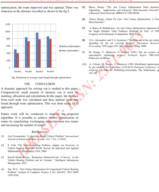
optimization, the route improved and was optimal. There was reduction in the distance travelled as shown in the fig.5.
Fig. Reduction in average route length through optimization
VIII. CONCLUSION
A dynamic approach for solving vrp is studied in this paper. Comparatively small amount of memory can is used for marking, allocation and calculations.In this paper, the distance from each node was calculated and then optimal route was found through route optimization. This was done using ACO approach.
Future work will be conducted to improve the proposed algorithm. It is possible to achieve further optimization of routes by transferring/ exchanging nodes between two routes and increasing the number of nodes.
REFERENCES
[1] Aziz Ezzatneshan “A algorithm for the Vehicle Problem” International Journal of Advanced Robotic Systems, Vol. 7, No. 2 (2010).
[2] P. Toth “The Vehicle Routing Problem, chapter An Overview of
Vehicle Routing Problems”SIAM, Society for Industrial and Applied
Mathematics, Philadelphia, USA, 2000.
[3] Suresh Nanda Kumar , Ramasamy Panneerselvam “A Survey on the Vehicle Routing Problemand its Variants “ Intelligent Information Management, 2012
[4] Tan, W.F., “Ant Colony Optimization for Capacitated Vehicle Routing Problem” Journal of Computer Science 8 (6): 846-852, 2012 ISSN 1549-3636.
[5] Marco Dorigo “The Ant Colony Optimization Meta heuristic:
Algorithms, Applications, and Advances” Meta heuristics Network”,
a Research Train Network, HPRN-CT-1999-00106.
[6] Marco Dorigo, Gianni Di Caro “Ant Colony Optimization: A New
Meta-Heuristic”.
[7] A. Bauer, B. Bullnheimer “An Ant Colony Optimization Approach for the Single Machine Total Tardiness Problem” In: Proc. of 1999
Congress on Evolutionary Computation. IEEE Press.
[8] D.A. Alexandrov and Y.A. Kochetov “The behavior of the ant colony
algorithm for the set covering problem” Operations Research Proceedings 1999, pages 255–260. Springer Verlag, 2000.
[9] M. Dorigo, V. Maniezzo, A. Colorni (1991) The ant system: an autocatalytic optimizing process, Technical Report TR91-016, Politecnico di Milano