A prediction based resampling method for estimating the number of clusters in a dataset

comment

reviews

reports

deposited research

interactions

information

refereed research

Research

A prediction-based resampling method for estimating the number

of clusters in a dataset

Sandrine Dudoit*

‡

_{and Jane Fridlyand}

†‡

Addresses: *Division of Biostatistics, School of Public Health, University of California Berkeley, 140 Earl Warren Hall, Berkeley, CA 94720-7360, USA. †_{Jain Lab, Comprehensive Cancer Center, University of California San Francisco, 2340 Sutter St, San Francisco, CA 94143-0128,}

USA. ‡_{Both authors contributed equally to this work.}

Correspondence: Sandrine Dudoit. E-mail: [email protected]

Abstract

Background: Microarray technology is increasingly being applied in biological and medical

research to address a wide range of problems, such as the classification of tumors. An important statistical problem associated with tumor classification is the identification of new tumor classes using gene-expression profiles. Two essential aspects of this clustering problem are: to estimate the number of clusters, if any, in a dataset; and to allocate tumor samples to these clusters, and assess the confidence of cluster assignments for individual samples. Here we address the first of these problems.

Results:We have developed a new prediction-based resampling method, Clest, to estimate the

number of clusters in a dataset. The performance of the new and existing methods were compared using simulated data and gene-expression data from four recently published cancer microarray studies. Clest was generally found to be more accurate and robust than the six existing methods considered in the study.

Conclusions:Focusing on prediction accuracy in conjunction with resampling produces accurate

and robust estimates of the number of clusters.

Published: 25 June 2002

GenomeBiology2002, 3(7):research0036.1–0036.21

The electronic version of this article is the complete one and can be found online at http://genomebiology.com/2002/3/7/research/0036 © 2002 Dudoit and Fridlyand, licensee BioMed Central Ltd (Print ISSN 1465-6906; Online ISSN 1465-6914)

Received: 18 February 2002 Revised: 22 April 2002 Accepted: 15 May 2002

Background

The burgeoning field of genomics, and in particular DNA microarray experiments, has revived interest in cluster analysis by raising new methodological and computational challenges. DNA microarrays are part of a new and promis-ing class of biotechnologies that allow the monitorpromis-ing of expression levels in cells for thousands of genes simultane-ously. Microarray experiments are increasingly being caried out in biological and medical research to address a wide range of problems, including the classification of tumors [1-6]. A reliable and precise classification of tumors is essen-tial for successful diagnosis and treatment of cancer. By allowing the monitoring of expression levels on a genomic

build predictors for new tumor samples. Inaccurate cluster assignments could lead to erroneous diagnoses and unsuit-able treatment protocols.

Here we address the estimation of the number of clusters in a dataset. First, we describe the basic principles of cluster analysis and review existing methods for estimating the number of clusters. We then present a new prediction-based resampling method, Clest, for estimating the number of clusters in a dataset. The performance of the new and exist-ing methods is compared usexist-ing simulated data and gene-expression data from four recently published cancer microarray studies. We have addressed the problem of improving and assessing the accuracy of a given clustering procedure in [7].

Cluster analysis

In classification, one is concerned with assigning objects to classes on the basis of measurements made on these objects. There are two main aspects to classification: discrimination and clustering, or supervised and unsupervised learning. In unsupervised learning (also known as cluster analysis, class discovery and unsupervised pattern recognition), the classes

are unknown a prioriand need to be discovered from the

data. In contrast, in supervised learning (also known as dis-criminant analysis, class prediction, and supervised pattern recognition), the classes are predefined and the task is to understand the basis for the classification from a set of labeled objects (training or learning set). This information is then used to classify future observations. The present article focuses on the unsupervised problem, that is, on cluster analysis, but draws on notions from supervised learning to address the problem.

In cluster analysis, the data are assumed to be sampled from

a mixture distribution with Kcomponents corresponding to

the K clusters to be recovered. Let (X1, ¼, Xp) denote a

random 1 x pvector of explanatory variables or features, and

let YÎ{1, ¼, K} denote the unknown component or cluster

label. Given a sample of Xvalues, the goal is to estimate the

number of clusters Kand to estimate, for each observation,

its cluster label Y.

Suppose we have data X= (xij) on pexplanatory variables

(for example, genes) for n observations (for example,

tumor mRNA samples), where xijdenotes the realization of

variable Xj for observation i and xi= (xi1,¼,xip) denotes

the data vector for observationi, i= 1,¼,n, j= 1,¼,p. We

consider clustering procedures that partition the learning

set L= {x₁,¼, x_n} into K clusters of observations that are

‘similar’ to each other, where K is a user-prespecified

integer. More specifically, the clustering P(·;L) assigns class

labels P(x_i;L) = ^y_ito each observation, where ^y_iÎ{1,¼,K}.

Clustering procedures generally operate on a matrix of pairwise dissimilarities (or similarities) between the observations to be clustered, such as the Euclidean or

Manhattan distance matrices [8]. A partitioning of the learning set can be produced directly by partitioning

clus-tering methods (for example, k-means, partitioning

around medoid (PAM), self-organizing maps (SOM)) or by hierarchical clustering methods, by ‘cutting’ the

dendro-gram to obtain K‘branches’ or clusters. Important issues,

which will only be addressed briefly in this article, include: the selection of observational units, the selection of vari-ables for defining the groupings, the transformation and standardization of variables, the choice of a similarity or dissimilarity measure, and the choice of a clustering method [9]. Our main concern here is to estimate the

number of clusters K.

When a clustering algorithm is applied to a set of observa-tions, a partition of the data is returned whether or not the data show a true clustering structure, that is, whether or not

K= 1. This fact causes no problems if clustering is done to

obtain a practical grouping of the given set of objects, as for organizational or visualization purposes (for example, hier-archical clustering for displaying large gene-expression data

matrices as in Eisen et al.[10]). However, if interest lies

pri-marily in the recognition of an unknown classification of the data, an artificial clustering is not satisfactory, and clusters resulting from the algorithm must be investigated for their relevance and reproducibility. This task can be carried out by descriptive and graphical exploratory methods, or by relying on probabilistic models and suitable statistical significance tests (for example [11,12]).

We argue here that validating the results of a clustering pro-cedure can be done effectively by focusing on prediction accuracy. Once new classes are identified and class labels are assigned to the observations, the next step is often to build a classifier for predicting the class of future observations. The reproducibility or predictability of cluster assignments becomes very important in this context, and therefore pro-vides a motivation for using ideas from supervised learning in an unsupervised setting. Resampling methods such as bagging [13] and boosting [14,15] have been applied success-fully in the field of supervised learning to improve prediction accuracy. We propose here a novel resampling method, Clest, which combines ideas from discriminant and cluster analysis for estimating the number of clusters in a dataset. Although the proposed resampling methods are applicable to general clustering problems and procedures, particular attention is given to the clustering of tumors on the basis of gene-expression data using the partitioning around medoids (PAM) procedure (see below).

Partitioning around medoids

comment

reviews

reports

deposited research

interactions

information

refereed research

number of clusters K. The PAM procedure is based on the

search forK representative objects, or medoids, among the

observations to be clustered. After finding a set of K

medoids,K clusters are constructed by assigning each

obser-vation to the nearest medoid. The goal is to findK medoids

that minimize the sum of the dissimilarities of the observa-tions to their closest medoid. The algorithm first looks for a good initial set of medoids, then finds a local minimum for the objective function, that is, a solution such that there is no single switch of an observation with a medoid that will decrease the objective.

The PAM method tends to be more robust and

computa-tionally efficient than k-means. In addition, PAM provides

a graphical display, the silhouette plot, which can be used to select the number of clusters and to assess how well

individual observations are clustered. Let ai denote the

average dissimilarity between iand all other observations

in the cluster to which i belongs. For any other cluster C,

let d(i,C) denote the average dissimilarity of ito all objects

of Cand let bidenote the smallest of these d(i,C). The

sil-houette width of observation i is sili= (bi- ai)/max(ai,bi)

and the overall average silhouette width is simply the

average of siliover all observations i, sil— = åisili/n.

Intu-itively, objects with large silhouette width siliare well

clus-tered, whereas those with small sili tend to lie between

clusters. Kaufman and Rousseeuw suggest estimating the

number of clusters K by that which gives the largest

average silhouette width,sil—.

Existing methods for estimating the number of clusters in a dataset

Null hypothesis

Suppose that the maximum possible number of clusters in the

data is set to M, 2 £M£n. One approach to estimating the

number of clustersK is to look for ^K, 1 < ^K£M, that provides

the strongest significant evidence against the null hypothesis

H0ofK = 1, that is, ‘no clusters’ in the data. Two commonly

used parametric null hypotheses are the unimodality hypothesis and the uniformity hypothesis.

Under the unimodality hypothesis, the data are thought to be a random sample from a multivariate normal distribu-tion. This model typically gives a high probability of

rejec-tion of the null K = 1 if the data are sampled from a

distribution with a lower kurtosis than the normal distribu-tion, such as the uniform distribution [17].

The uniformity hypothesis, also referred to as random posi-tion hypothesis, states that the data are sampled from a

uniform distribution in p-dimensional space [18-20].

Methods based on the uniformity hypothesis tend to be con-servative, that is, lead to few rejections of the null hypothe-sis, when the data are sampled from a strongly unimodal distribution such as the normal distribution. In two or more dimensions, and depending on the test statistic, the results

can be very sensitive to the region of support of the reference distribution [17].

For both types of hypotheses, evidence against the null hypothesis can be summarized formally under probability models for the data or more informally by using internal indices as described next.

Internal indices

Numerous methods have been proposed for testing the

null hypothesisK = 1 and estimating the number of

clus-ters in a dataset, however, none of them is completely sat-isfactory. Jain and Dubes [20] provide a general overview of such methods. The majority of existing approaches do

not attempt to formally test the null hypothesis thatK = 1,

but rather look for the clustering structure under which a summary statistic of interest is optimal, being large or small depending on the statistic [21-23]. These statistics are typically functions of the within-clusters, and possibly between-clusters, sums of squares. They are referred to as internal indices, in the sense that they are computed from the same observations that are used to create the cluster-ing. Consequently, the distribution of these indices is intractable. In particular, as clustering methods attempt to maximize the separation between clusters, the ordinary

significance tests such as analysis of variance F-tests are

not valid for testing differences between the clusters. Milli-gan and Cooper [12] conducted an extensive Monte Carlo evaluation of 30 internal indices. Other approaches include modeling the data using Gaussian mixtures and applying a Bayesian criterion to determine the number of components in the mixture [11]. A recent proposal of

Tib-shirani et al. [24], called the gap statistic method,

cali-brates an internal index, such as the within-clusters sum of squares, against its expectation under a suitably defined null hypothesis (note that gap tests have been used in another context in cluster analysis by Bock [18] to test the null hypothesis of a ‘homogeneous’ population against the

alternative of ‘heterogeneity’). Tibshirani et al.carried out

a comparative Monte Carlo study of the gap statistic and several of the internal indices that showed a better perfor-mance in the study of Milligan and Cooper [12]. These internal indices and the gap statistic are described in more detail below.

For a given partition of the learning set into 1 £k£M

clus-ters, define Bkand Wkto be the px pmatrices of between

and within k-clusters sums of squares and cross-products

[8]. Note that B1is not defined. The following six internal

indices are commonly used to estimate the number of

clus-ters in a dataset.

sil: Kaufman and Rousseeuw [16] suggest selecting the

number of clusters k³2 which gives the largest average

sil-houette width, sil—k. Silhouette widths were defined above

ch: Calinski and Harabasz [21]. For each number of clusters

k³2, define the index

trBk/(k- 1)

chk= ————————,

trWk/(n- k)

where tr denotes the trace of a matrix, that is, the sum of the diagonal entries. The estimated number of clusters is

argmaxk³2chk.

kl: Krzanowski and Lai [23]. For each number of clusters

k³2, define the indices

diffk= (k- 1)2/ptrWk-1- k2/ptrWk and

klk= | diffk |/|diffk+1|.

The estimated number of clusters is argmaxk³2klk.

hart: Hartigan [25]. For each number of clusters k ³ 1,

define the index

trWk

hartk=

trWk+1

The estimated number of clusters is the smallest k³1 such

that hartk£10.

gapor gapPC: Tibshirani et al.[24]. This method compares an observed internal index, such as the within-clusters sum of squares, to its expectation under a reference null

distribu-tion as follows. For each number of clusters k³1, compute

the within-clusters sum of squares trWk. Generate B(here

B= 10) reference datasets under the null distribution and

apply the clustering algorithm to each, calculating the

within-clusters sums of squares trWk1, ¼, trWkB. Compute

the estimated gap statistic

gapk= —_B 1

b log tr W

b

k- log tr Wk

and the standard deviation sdkof log trWkb, 1 £b£ B. Let

sd~k= sdkÖ[(1 + 1/B)]. The estimated number of clusters is

the smallest k³1 such that gapk³ gapk*- sd~k*, where k* =

argmaxk³1gapk.

Tibshirani et al. [24] chose the uniformity hypothesis to

create a reference null distribution and considered two approaches for constructing the region of support of the dis-tribution. In the first approach, the sampling window for the

jth variable, 1 £j£p, is the range of the observed values for

that variable. In the second approach, following Sarle [17], the variables are sampled from a uniform distribution over a box aligned with the principal components of the centered

design matrix (that is, the columns of Xare first set to have

mean 0 and the singular value decomposition of Xis

com-puted). The new design matrix is then back-transformed to obtain a reference dataset. Whereas the first approach has the advantage of simplicity, the second takes into account the shape of the data distribution. Note that in both approaches the variables are sampled independently. The version of the gap method that uses the original variables to construct the region of support is referred to as gap and the second version as gapPC, where ‘PC’ stands for princi-pal components.

Note that of the above methods, only hart, gap, and gapPC allow the estimation of only one cluster in the data, that is, ^

K = 1.

External indices

The term ‘validation of a clustering procedure’ usually refers to the ability of a given method to recover the true clustering structure in a dataset. There have been several attempts to assess validity on theoretical grounds [18,25]; however, such approaches turn out to be of little applicability in the context of high-dimensional complex datasets. In many validation studies, clustering methods are evaluated on their

perfor-mance on empirical datasets with a priori known cluster

labels [25] or, more commonly, on simulation studies where true cluster labels are known. To assess the ability of a clus-tering procedure to recover true cluster labels it is necessary to define a measure of agreement between two partitions;

the first partition being the a prioriknown clustering

struc-ture of the data, and the second partition resulting from the clustering procedure. In the clustering literature, measures of agreement between partitions are referred to as external indices; several such indices are reviewed next.

Consider two partitions of nobjects x1, ¼, xn: the R-class

parti-tion U= {u1, ¼, uR} and the C-class partition V= {v1, ¼, vC}.

External indices of partitional agreement can be expressed

in terms of a contingency table (Table 1), with entry nij

denoting the number of objects that are both in clusters ui

and vj, i = 1,¼,R, j = 1,¼,C[20]. Let ni.= åjC= 1 nij and

n.j=åRi= 1nijdenote the row and column sums of the

contin-gency table, respectively, and let Z= åR

i= 1åCj= 1nij2.

Table 1

Contingency table for two partitions of nobjects

v₁ v₂ ¼ v_C

u₁ n₁₁ n₁₂ ¼ n_1C n_1.

u₂ n₂₁ n₂₂ ¼ n_2C n_2.

u_R n_R1 n_R2 ¼ n_RC n_R.

n_.1 n_.2 ¼ n_.C n_{. .}= n

The following indices can then be used.

1. Rand:Rand [26]

Rand= 1 +

i=1n 2

i. +

C

j=1n 2

.j )

2. Jaccard: Jain and Dubes [20]

Jac=

i=1n 2

i. +

C

j=1n 2

.j - Z- n

3. FM:Fowlkes and Mallows [27]

FM=

i=1

ni.

2

C

j=1

n.j

2 ½.

Note that Rand and FM are linear functions of Z, and hence

are linear functions of one another, conditional on the row and column sums in Table 1. If the row and column sums in Table 1 are fixed, but the partitions are selected at random; that is, if there is independence in the table, the hypergeo-metric distribution can be applied to determine the expected

value of quantities such as Z. In particular

E

i=1

C

j=1

nij

2

R

i=1

ni.

2

C

j=1

n.j

2 n2

An external index S is often standardized in such a way that its expected value is 0 when the partitions are selected at random and 1 when they match perfectly. This amounts to computing a standardized external index

S -E(S)

S¢= ———————,

Smax- E(S)

where Smaxis the maximum value of the statistic Sand E(S)

is the expected value of Swhen partitions are selected at

random. Accordingly, an often used correction for the Rand statistic is

i=1

Rand¢= ———————————————————————————————.

(1/2)

2

C

j=1

The significance of an observed external index is usually assessed under the assumption that the two partitions to be compared are independent. This assumption does not hold for the resampling methods described in the following section, since the same data are used to produce the two par-titions. Nevertheless, external indices are convenient tools for comparing two clusterings, and are used in the new resampling method Clest. In this context, one should think of these indices as internal rather than external measures.

Results

Clest, a prediction-based resampling method for estimating the number of clusters

We propose a new prediction-based resampling method, Clest, for estimating the number of clusters, if any, in a dataset. The idea behind Clest is very intuitive if one is concerned with reproducibility or predictability of cluster assignments.

It is proposed to estimate the number of clusters K by

repeatedly randomly dividing the original dataset into two

non-overlapping sets, a learning set Lband a test set Tb. For

each iteration and for each number of clusters k, a clustering

P(·;Lb) of the learning set Lb is obtained and a predictor

C(·;Lb) is built using the class labels from the clustering. The

predictor C(·;Lb) is then applied to the test set Tb and the

predicted labels are compared to those produced by applying the clustering procedure to the test set, using one of the external indices (or similarity statistics) described in the Background section. The number of clusters is estimated by

comparing the observed similarity statistic for each kto its

expected value under a suitable null distribution withK = 1.

The estimated number of clusters is defined to be the ^K

cor-responding to the largest significant evidence against the

null hypothesis ofK = 1.

An early version of this approach was introduced by Breck-enridge [28] under the name of replication analysis and was designed to evaluate the stability of a clustering. In the

origi-nal replication aorigi-nalysis, the number of clusters k is fixed,

and the data are randomly divided into two samples. A

clus-tering procedure partitions both samples into kclusters, and

the centroids of the clusters of the first sample are com-puted. A second set of labels is assigned to the observations in the second sample by assigning to each observation the cluster label of the closest centroid from the first sample. Finally, an external index is used to assess the agreement between the two partitions of the second sample. This measure reflects the stability of the clustering structure. The Clest procedure proposed here generalizes the work of Breckenridge [28].

Clest procedure for estimating the number of clusters in a dataset

Denote the maximum possible number of clusters by M,

2£M£n. For each number of clusters k, 2 £k£M, perform

steps 1-4.

1. Repeat the following Btimes:

(a) Randomly split the original learning set Linto two

non-overlapping sets, a learning set Lband a test set Tb.

(b) Apply a clustering procedure Pto the learning set Lbto

obtain a partition P(·;Lb).

(c) Build a classifier C(·;Lb) using the learning set Lband its

cluster labels.

(d) Apply the resulting classifier to the test set Tb.

comment

reviews

reports

deposited research

interactions

information

(e) Apply the clustering procedure P to the test set Tbto

obtain a partition P(·;Tb).

(f) Compute an external index sk,bcomparing the two sets

of labels for Tb, namely the labels obtained by clustering

and prediction.

2. Let tk= median(sk,1, ¼, sk,B) denote the observed

similar-ity statistic for the k-cluster partition of the data.

3. Generate B0 datasets under a suitable null hypothesis.

For each reference dataset, repeat the procedure described

in steps 1 and 2 above, to obtain B0 similarity statistics

tk,1, ¼, tk,B0.

4. Let t0

k denote the average of these B0 statistics, t0k =

[1/(B0)]åbB0=1tk,b, and let pkdenote the proportion of the tk,b,

1£b£B0, that are at least as large as the observed statistic

tk, that is, the p-value for tk. Finally, let dk= tk- t0kdenote the

difference between the observed similarity statistic and its

estimated expected value under the null hypothesis ofK = 1.

Define the set Kas

K-_{= {2ⱕkⱕM : p}

kⱕpmax,dkⱖdmin},

where pmaxand dminare preset thresholds (see Parameters of

the Clest procedure section below). If this set is empty,

esti-mate the number of clusters as ^K = 1. Otherwise, let

^

K= argmaxkÎK-dk, that is, take the number of clusters ^Kthat

corresponds to the largest significant difference statistic dk.

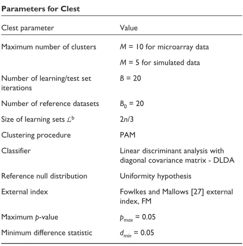
Parameters of the Clest procedure

In this paper, the following decisions are made regarding the different parameters for the Clest procedure (see summary in Table 2).

Clustering procedure: partitioning around medoids (PAM)

The PAM clustering procedure of Kaufman and Rousseeuw [16], implemented in the cluster package in R and S-Plus, was used to cluster observations based on the Euclidean dis-tance metric (see Background).

Classifier: diagonal linear discriminant analysis (DLDA)

For multivariate Gaussian class conditional densities, that is,

for x|y = k ~ N(mk,Sk), the maximum likelihood (ML)

dis-criminant rule (or Bayes rule with uniform class priors)

pre-dicts the class of an observation xby that which gives the

largest likelihood to x, that is,

C(x) = argmin1ⱕkⱕK

When the class densities have the same diagonal covariance

matrix S= diag(s12,¼,sp2), the discriminant rule is linear and

given by

(xj- mkj)2

C(x) = argmin_1ⱕkⱕK

p

j=1————— .s2_j

For the corresponding sample ML discriminant rules, the population mean vectors and covariance matrices are esti-mated from a learning set by the sample mean vectors and

covariance matrices, respectively: ^mk = x–k and ^SSk= Sk. For

the constant covariance matrix case, the pooled estimate of the

common covariance matrix is used: ^SS = åk(nk-1 ) Sk/(n- K),

where nkdenotes the number of observations in class kand n

is the total sample size. DLDA is a very simple classifier but it has been shown to perform well in complex situations, in par-ticular, in an extensive study of discrimination methods for the classification of tumors using gene-expression data [29]. DLDA is also known as naive Bayes classification.

Reference null distribution

The reference datasets are generated under the uniformity hypothesis as in the gap statistic method (see Background).

External index

All the external indices described in Background were con-sidered. The FM index [27] was found to be superior to the other indices when reference datasets are generated under the uniformity hypothesis (data not shown).

Threshold parameters,p_maxand d_min

The choices pmax= 0.05 and dmin= 0.05 are ad hocand can

probably be improved upon. Nevertheless, this rule gives a satisfactory performance and is used in the absence of a better choice.

Table 2

Parameters for Clest

Clest parameter Value

Maximum number of clusters M= 10 for microarray data M= 5 for simulated data Number of learning/test set B= 20

iterations

Number of reference datasets B₀= 20 Size of learning sets Lb _2n/3

Clustering procedure PAM

Classifier Linear discriminant analysis with diagonal covariance matrix - DLDA Reference null distribution Uniformity hypothesis

External index Fowlkes and Mallows [27] external index, FM

Number of iterations and reference datasets

Here we used B= B0= 20. In general, the Clest procedure is

robust to the choice of Band B0(data not shown).

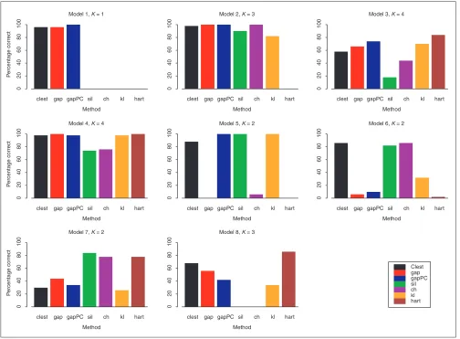
Comparison of procedures on simulated data

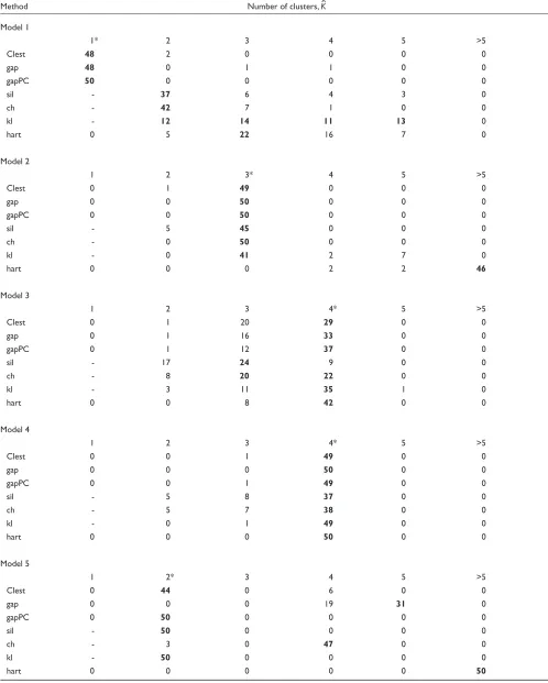
The new procedure Clest was compared to six existing methods presented in Background using data simulated from the models described in Materials and methods. Figure 1 displays bar plots for the percentage of simulations for which a given method correctly recovered the number of clusters for each of the eight models. Table 3 provides a more detailed account of the simulation results for each pro-cedure. It can be seen that Clest gave uniformly good results over the range of models, its worst performance being for Model 7 with two overlapping clusters. The rest of the methods failed for at least one of the eight models consid-ered. The gap procedure failed twice (Models 5 and 6) and gapPC failed once (Model 6). Neither gap nor gapPC were

able to identify the presence of the two clusters for Model 6, which is a model with two drawn-out clusters and seven noise variables with varying variances. Both gap and gapPC consistently estimated one cluster for this model, perhaps because both methods are based on the within-clusters sums of squares and consequently are more affected by the vari-ables with larger variances. In a majority of the simulations from Model 7, Clest, gap, and gapPC failed to distinguish between one and two clusters, while the simple hart index performed well. The rest of the procedures do not have, by definition, the ability to estimate one cluster and hence gen-erally identified the two clusters. Interestingly, for Model 8 with three overlapping clusters, sil and ch performed poorly, choosing two clusters in a majority of the simulations, while hart and Clest showed the best performance. Overall, most methods tended to underestimate more often than they overestimated the number of clusters, but the situation was reversed for hart and kl. For Model 1 it is only fair to

comment

reviews

reports

deposited research

interactions

information

refereed research

Figure 1

Estimating the number of clusters; results for simulated data. For each of the eight simulation models, the bar plots represent the percentage of simulations for which the number of clusters was correctly estimated by each method (out of 50 simulations).

clest gap gapPC sil ch kl hart

0

2

04

06

08

0

1

0

0

Method

P

ercentage correct

P

ercentage correct

P

ercentage correct

Model 1, K = 1

clest gap gapPC sil ch kl hart

0

2

04

06

08

0

1

0

0

Method Model 2, K = 3

clest gap gapPC sil ch kl hart

0

2

04

06

08

0

1

0

0

Method Model 3, K = 4

clest gap gapPC sil ch kl hart

0

20

40

60

80

100

Method Model 4, K = 4

clest gap gapPC sil ch kl hart

0

20

40

60

80

100

Method Model 5, K = 2

clest gap gapPC sil ch kl hart

0

20

40

60

80

100

Method Model 6, K = 2

clest gap gapPC sil ch kl hart

0

20

40

60

80

100

Method Model 7, K = 2

clest gap gapPC sil ch kl hart

0

20

40

60

80

100

Method Model 8, K = 3

Table 3

Estimating the number of clusters in simulated data

Method Number of clusters, K^

Model 1

1* 2 3 4 5 >5

Clest 48 2 0 0 0 0

gap 48 0 1 1 0 0

gapPC 50 0 0 0 0 0

sil - 37 6 4 3 0

ch - 42 7 1 0 0

kl - 12 14 11 13 0

hart 0 5 22 16 7 0

Model 2

1 2 3* 4 5 >5

Clest 0 1 49 0 0 0

gap 0 0 50 0 0 0

gapPC 0 0 50 0 0 0

sil - 5 45 0 0 0

ch - 0 50 0 0 0

kl - 0 41 2 7 0

hart 0 0 0 2 2 46

Model 3

1 2 3 4* 5 >5

Clest 0 1 20 29 0 0

gap 0 1 16 33 0 0

gapPC 0 1 12 37 0 0

sil - 17 24 9 0 0

ch - 8 20 22 0 0

kl - 3 11 35 1 0

hart 0 0 8 42 0 0

Model 4

1 2 3 4* 5 >5

Clest 0 0 1 49 0 0

gap 0 0 0 50 0 0

gapPC 0 0 1 49 0 0

sil - 5 8 37 0 0

ch - 5 7 38 0 0

kl - 0 1 49 0 0

hart 0 0 0 50 0 0

Model 5

1 2* 3 4 5 >5

Clest 0 44 0 6 0 0

gap 0 0 0 19 31 0

gapPC 0 50 0 0 0 0

sil - 50 0 0 0 0

ch - 3 0 47 0 0

kl - 50 0 0 0 0

compare Clest, gap, gapPC, and hart, as the other methods

only estimate ^K³2.

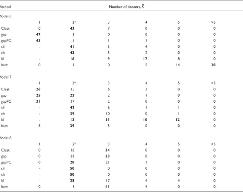
In summary, for the simulation models considered here, Clest was the most robust and accurate, whereas hart per-formed worst. gapPC was better than gap and the rest of the methods performed similarly.

For a given model, it is of interest to consider the median value of the statistics used by each method to estimate the

number of clusters. For each number of clusters k, the plots

of the median values, over the 50 simulated datasets, of the

Clest dk-statistic, gapPCk, and

—

silk statistics are shown in

Figures 2, 3 and 4, respectively. The d-statistic does not

gen-erally have local maxima except for Model 5. There, a local

maximum appears at K = 4 clusters, but the global

maximum occurs atK = 2. It can be seen that the ability of

Clest to distinguish between one and two clusters is very low

for Model 7; the median of the d2values is less than the

sig-nificance cut-off dminused in the Clest procedure. Indeed,

the results in Table 3 show that Clest identified two clusters for only 30% of the datasets simulated from Model 7. The figures suggest that for the majority of the models, the global

maximum of the median dk-statistic is more pronounced

than the global maxima of the median gapPCkand

—

silk

sta-tistics, respectively. This again suggests good robustness and accuracy properties for the Clest method.

Comparison of procedures on microarray data

The new Clest method was also evaluated using gene-expres-sion data from the four cancer microarray studies described in Materials and methods and summarized in Table 4. Recall that mRNA samples in the lymphoma, leukemia, and NCI60 datasets were assigned class labels from the laboratory

comment

reviews

reports

deposited research

interactions

information

refereed research

Table 3 (continued)

Method Number of clusters, K^

Model 6

1 2* 3 4 5 >5

Clest 0 43 7 0 0 0

gap 47 3 0 0 0 0

gapPC 43 5 1 1 0 0

sil - 41 5 4 0 0

ch - 43 5 2 0 0

kl - 16 9 17 8 0

hart 0 1 0 5 14 30

Model 7

1 2* 3 4 5 >5

Clest 26 15 6 3 0 0

gap 25 22 2 1 0 0

gapPC 31 17 2 0 0 0

sil - 42 6 1 1 0

ch - 39 10 0 1 0

kl - 13 15 10 12 0

hart 6 39 5 0 0 0

Model 8

1 2* 3 4 5 >5

Clest 0 16 34 0 0 0

gap 0 22 28 0 0 0

gapPC 0 28 21 1 0 0

sil - 50 0 0 0 0

ch - 50 0 0 0 0

kl - 25 17 4 4 0

hart 0 3 43 4 0 0

analyses of the tumor samples or from a prioriknowledge of the cell lines. For the melanoma dataset, tumor class labels were obtained from the statistical analysis described in

Bittner et al.[30]. In the discussion that follows, these class

labels are treated as known. The six methods described in Background and Clest were applied to estimate the number of clusters for each of the four microarray datasets; the results are presented in Table 5.

The methods Clest and sil correctly estimated the presumed number of classes for all but the NCI60 dataset, where both methods identified three clusters only. The gap and gapPC methods overestimated the number of clusters for all datasets, with the exception of gapPC, which identified eight clusters for the NCI60 dataset. The ch method estimated two clusters for each of the four datasets, whereas kl and hart identified four classes for the lymphoma dataset.

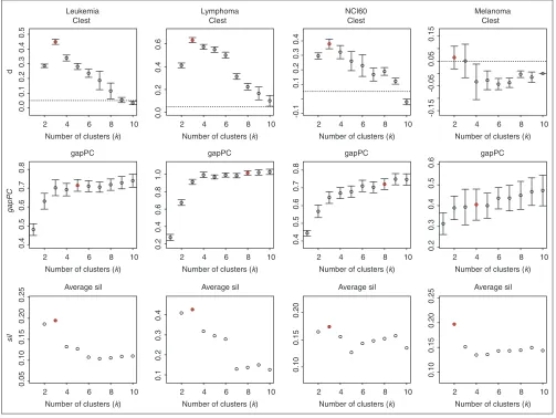
For Clest, gapPC, and sil, we further investigated how the strength of the evidence for the estimated number of clusters

varied between datasets. Figure 5 displays plots of the dk,

gapPCk, and sil—kstatistics versus the number of clusters k.

Error bars for dkand gapPCkare based on the standard

devi-ations of tkand log trWkunder their respective null

distribu-tions. Whereas the evidence for the existence of clusters is very strong for the lymphoma, leukemia, and NCI60 datasets, the evidence for the two clusters in the melanoma dataset is much weaker. In particular, for Clest, the maximum value of

the dkstatistic barely reaches the dminthreshold of 0.05. For

the leukemia dataset, the dk statistic clearly peaks at k = 3

clusters and drops off abruptly; for the lymphoma and NCI60 datasets the decrease is more gradual. Note that according to Clest there was not enough evidence to identify the two DLBCL subclasses for the lymphoma dataset. Alizadeh

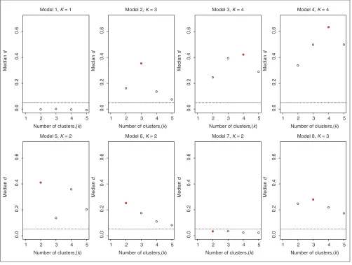
et al. [1] identified these subclasses using subject matter Figure 2

Estimating the number of clusters using the Clest procedure; results for simulated data. Plots are of median d_kversus kfor each simulation model (medians are computed over 50 simulations). The horizontal line corresponds to the d_mincut-off of 0.05, and the true number of clusters is indicated by a filled plotting symbol.

Number of clusters,(k)

Median

d

1 2 3 4 5

0.0

0.2

0.4

0.6

Model 1, K = 1

Number of clusters,(k)

1 2 3 4 5

0.0

0.2

0.4

0.6

Model 2, K = 3

Number of clusters,(k)

1 2 3 4 5

0.0

0.2

0.4

0.6

Model 3, K = 4

Number of clusters,(k)

1 2 3 4 5

0.0

0.2

0.4

0.6

Model 4, K = 4

Number of clusters,(k)

Median

d

Median

d

Median

d

Median

d

Median

d

Median

d

Median

d

1 2 3 4 5

0.0

0.2

0.4

0.6

Model 5, K = 2

Number of clusters,(k)

1 2 3 4 5

0.0

0.2

0.4

0.6

Model 6, K = 2

Number of clusters,(k)

1 2 3 4 5

0.0

0.2

0.4

0.6

Model 7, K = 2

Number of clusters,(k)

1 2 3 4 5

0.0

0.2

0.4

0.6

knowledge to select the genes for the clustering procedure; here the genes were selected in an unsupervised manner.

Discussion

Resampling methods such as bagging and boosting have been applied successfully in a supervised learning context to improve prediction accuracy. Here and in a related article [7], we have proposed resampling methods to address two main problems in cluster analysis: estimating the number of clusters, if any, in a dataset; improving and assessing the accuracy of a given clustering procedure. As the groups obtained from cluster analysis are often used later on for prediction purposes, the approaches to these two problems rely on and extend ideas from supervised learning. Although the methods are applicable to general clustering problems and procedures, particular attention is given to the clustering of

tumors using gene-expression data. The performance of the proposed and existing methods was compared using simulated data and gene-expression data from four recently published cancer microarray studies.

To estimate the number of clusters in a dataset, we propose a prediction-based resampling method, Clest, which estimates

the number of clusters K based on the reproducibility of

cluster assignments. In comparative studies, Clest was gen-erally found to be more accurate and robust than six existing methods. For the simulated datasets, Clest performed well across a wide range of models with varying numbers of over-lapping and non-overover-lapping clusters, different numbers of variables and covariance matrix structures. Unlike methods based on between- or within-clusters sums of squares, the resampling method seems robust to the varying covariance structure of the variables.

comment

reviews

reports

deposited research

interactions

information

refereed research

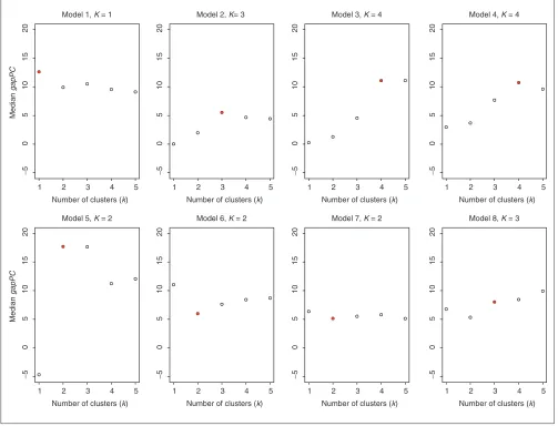
Figure 3

Estimating the number of clusters using the gapPC procedure; results for simulated data. Plots are of median gapPC_kversus kfor each simulation model (medians are computed over 50 simulations). The true number of clusters is indicated by a filled plotting symbol.

Number of clusters (k)

Median

gapPC

1 2 3 4 5

−

5

05

10

15

20

Model 1, K = 1

Number of clusters (k)

1 2 3 4 5

−

50

5

1

0

1

5

2

0

Model 2, K= 3

Number of clusters (k)

1 2 3 4 5

−

50

5

1

0

1

5

2

0

Model 3, K = 4

Number of clusters (k)

1 2 3 4 5

−

50

5

1

0

1

5

2

0

Model 4, K = 4

Number of clusters (k)

Median

gapPC

1 2 3 4 5

−

5

05

1

0

15

20

Model 5, K = 2

Number of clusters (k)

1 2 3 4 5

−

50

5

1

0

1

5

2

0

Model 6, K = 2

Number of clusters (k)

1 2 3 4 5

−

50

5

1

0

1

5

2

0

Model 7, K = 2

Number of clusters (k)

1 2 3 4 5

−

50

5

1

0

1

5

2

0

For the microarray datasets, Clest and sil correctly estimated the number of tumor or cell-line clusters (as determined

from a prioriknown or putative tumor and cell-line classes)

for three out of the four datasets; the performance of other methods was significantly worse. We focus here on the clus-tering of tumor mRNA samples using gene-expression data. Once tumor classes are specified, an important next step would be the identification of marker genes that characterize these different tumor classes. A related question, which we have not considered here, is the ‘transpose’ clustering problem; that is, the clustering of genes that have similar expression levels across biological samples. One could then investigate the clusters for the presence of shared regulatory motifs among the genes [31]. This could lead to the identifi-cation of genes that are not only coexpressed but are also under similar regulatory control. Joint analysis of transcript level and sequence data should lead to greater biological insight into the molecular characterization of tumors.

A number of decisions were made regarding the different parameters of the Clest procedure. The clustering procedure PAM was used in the comparison; however, one should keep in mind that different clustering procedures can generate different partitions of the same data, possibly leading to dif-ferent inferences about the number of clusters. In addition, the clustering (PAM) and prediction methods (DLDA or naive Bayes) considered in this article focus on similar fea-tures of the data, namely, the distance of the observations from cluster ‘centers’. More work is needed to investigate the robustness of Clest to these choices. In particular, it would be interesting to consider prediction and clustering methods that focus on different aspects of the data (for example, clas-sification trees instead of DLDA). Although it may seem that having a classifier as a parameter of the Clest procedure creates more room for error, we have found that this is not the case in practice. When the classifier in Clest performs poorly, other methods for estimating the number of clusters Figure 4

Estimating the number of clusters using the sil procedure; results for simulated data. Plots are of median sil–kversus k for each simulation model (medians

are computed over 50 simulations). The true number of clusters is indicated by a filled plotting symbol.

Number of clusters (k)

Median

sil

Median

sil

1 2 3 4 5

0.0

0.2

0.4

0.6

0.8

1.0

Model 1, K = 1

Number of clusters (k)

1 2 3 4 5

0.0

0.2

0.4

0.6

0.8

1.0

Model 2, K = 3

Number of clusters (k)

1 2 3 4 5

0.0

0.2

0.4

0.6

0.8

1.0

Model 3, K = 4

Number of clusters (k)

1 2 3 4 5

0.0

0.2

0.4

0.6

0.8

1.0

Model 4, K = 4

Number of clusters (k)

1 2 3 4 5

0.0

0.2

0.4

0.6

0.8

1.0

Model 5, K = 2

Number of clusters (k)

1 2 3 4 5

0.0

0.2

0.4

0.6

0.8

1.0

Model 6, K = 2

Number of clusters (k)

1 2 3 4 5

0.0

0.2

0.4

0.6

0.8

1.0

Model 7, K = 2

Number of clusters (k)

1 2 3 4 5

0.0

0.2

0.4

0.6

0.8

1.0

also perform poorly. Another important choice in the Clest procedure is the reference null distribution used to calibrate

the observed similarity statistics tkfor different numbers of

clusters. The uniformity hypothesis was used here; a natural alternative would be to consider random permutations of the variables, that is, permutations of the entries of the design matrix within columns. In Clest, the observed similarity

sta-tistics tkare compared across numbers of clusters kby

con-sidering their distance from their estimated expected value

t0

k under the null distribution. A more sensitive calibration

may be achieved by taking scale into account, that is, by

dividing the difference statistic dkby the standard deviation

of tk under the null distribution, or even by considering

p-values pkfor tk. We briefly considered these refinements

and found that on their own they did not allow good

discrim-ination between the different ks. The Clest method does,

however, use the idea of p-value in combination with the

dif-ferences dk, as it imposes an upper limit on the p-value pk.

Finally, the choice of cut-off parameters dminand pmaxwas

rather ad hocand could be fine tuned.

We have not considered model-based methods, such as the Bayesian approach of Fraley and Raftery [11] or the

mixture-model approach of McLachlan et al.[32]. Another issue only

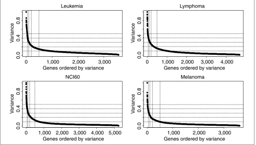
briefly addressed here is the selection of variables on which to base the clusterings. For the microarray datasets, genes were selected on the basis of the variance of their expression levels across samples, and it was found that the clusterings were fairly robust to the number of genes.

Resampling methods are promising tools for addressing

various problems in cluster analysis. Ben-Hur et al. [33]

have recently proposed a stability-based method for estimat-ing the number of clusters, where stability is characterized by the distribution of pairwise similarities between cluster-ings obtained from subsamples of the data. It would be

interesting to relate the approach of Ben-Hur et al. and

Clest. Elsewhere, we proposed two bagged clustering methods for improving and assessing the accuracy of a given partitioning clustering procedure [7]. There, the bootstrap is used to generate and aggregate multiple clusterings and to assess the confidence of cluster assignments for individual observations. Leisch [34] proposed a bagged clustering method which is a combination of partitioning and hierar-chical methods. A partitioning method is applied to boot-strap learning sets and the resulting partitions are combined by performing hierarchical clustering of the cluster centers. This method is similar in spirit to our two new bagging pro-cedures [7].

Conclusions

Focusing on prediction accuracy in conjunction with resam-pling produces accurate and robust estimates of the number of clusters. As reproducibility of the cluster assignments is an integral part of the Clest method, the clustering results can be used reliably for building a classifier to predict the class of future observations. In addition, the procedure is robust to the covariance structure among variables.

Materials and methods

Simulation models

Procedures for estimating the number of clusters in a dataset were evaluated using simulated data from a variety of

models, including those considered by Tibshirani et al.[24].

The models used for comparison contain different numbers of overlapping and non-overlapping clusters, different numbers of variables, and a wide range of covariance matrix structures. In addition, a variable number of irrelevant or ‘noise’ variables are included in the models. A noise variable is a variable whose distribution does not depend on the

comment

reviews

reports

deposited research

interactions

information

refereed research

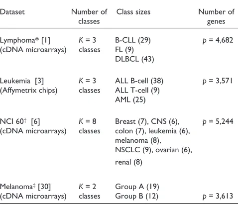
Table 4

Description of microarray datasets

Dataset Number of Class sizes Number of

classes genes

Lymphoma*[1] K= 3 B-CLL (29) p= 4,682 (cDNA microarrays) classes FL (9)

DLBCL (43)

Leukemia [3] K= 3 ALL B-cell (38) p= 3,571 (Affymetrix chips) classes ALL T-cell (9)

AML (25)

NCI 60† _{[6] K= 8 Breast (7), CNS (6), p= 5,244}

(cDNA microarrays) classes colon (7), leukemia (6), melanoma (8), NSCLC (9), ovarian (6), renal (8)

Melanoma‡_{[30] K= 2 Group A (19)}

(cDNA microarrays) classes Group B (12) p= 3,613 *The DLBCL class for the lymphoma dataset is likely to contain two subclasses.†_{For the NCI60 data, the two prostate cell lines and the}

unknown cell line (ADR-RES) were excluded from our analysis because of their small class size. ‡_{Note that for the first three datasets, tumor classes}

were known a priori, whereas for the melanoma dataset the two classes were inferred by Bittner et al.[30] by cluster analysis but not confirmed on an independent dataset.

Table 5

Estimating the number of clusters from microarray data Dataset Known Clest gap gapPC sil ch kl hart

Lymphoma 3 3 10 8 3 2 4 4

Leukemia 3 3 10 5 3 2 3 3

NCI60 8 3 10 8 3 2 6 2

cluster label, and such variables are added to obscure the underlying clustering structure to be recovered.

Model 1.One cluster in 10 dimensions. n= 200 observa-tions are simulated from the uniform distribution over the

unit hypercube in p= 10 dimensions.

Model 2. Three clusters in two dimensions. The observa-tions in each of the three clusters are independent bivariate normal random variables with means (0,0), (0,5), and (5,-3), respectively, and identity covariance matrix. There are 25, 25, and 50 observations in each of the 3 clusters, respectively.

Model 3.Four clusters in 10 dimensions, 7 noise variables. Each cluster is randomly chosen to have 25 or 50 observa-tions, and the observations in a given cluster are indepen-dently drawn from a multivariate normal distribution with identity covariance matrix. For each cluster, the cluster

means for the first three variables are randomly chosen from

a N(03, 25I3) distribution, where 0pdenotes a 1 x pvector of

zeros and Ipdenotes the p xpidentity matrix. The means for

the remaining seven variables are 0. Any simulation where the Euclidean distance between the two closest observations belonging to different clusters is less than 1 is discarded.

Model 4.Four clusters in 10 dimensions. Each cluster is randomly chosen to contain 25 or 50 observations, with

means randomly chosen as N(010, 3.6I10). The observations

in a given cluster are independently drawn from a normal distribution with identity covariance matrix and appropriate mean vector. Any simulation where the Euclidean distance between the two closest observations belonging to different clusters is less than 1 is discarded.

Model 5. Two elongated clusters in three dimensions. Cluster 1 contains 100 observations generated as follows. Set Figure 5

Estimating the number of clusters; results for microarray data. Plots of d_k, gapPC_k, and sil–_kversus k, with error bars computed as described in Results. The horizontal lines for the d_kplots correspond to a d_mincut-off of 0.05. The estimates for the number of clusters are indicated by filled plotting symbols.

Leukemia Clest

Number of clusters (k)

d

2 4 6 8 10

0.0

0.1

0.2

0.3

0.4

0.5

gapPC

Number of clusters (k)

gapPC

2 4 6 8 10

0.4

0.5

0.6

0.7

0.8

Average sil

Number of clusters (k)

sil

2 4 6 8 10

0.05

0.10

0.15

0.20

0.25

Lymphoma Clest

Number of clusters (k)

2 4 6 8 10

0.0

0.2

0.4

0.6

gapPC

Number of clusters (k)

2 4 6 8 10

0.2

0.4

0.6

0.8

1.0

Average sil

Number of clusters (k)

2 4 6 8 10

0.1

0.2

0.3

0.4

NCI60 Clest

Number of clusters (k)

2 4 6 8 10

-0.1

0.1

0.2

0.3

0.4

gapPC

Number of clusters (k)

2 4 6 8 10

0.4

0.5

0.6

0.7

0.8

Average sil

Number of clusters (k)

2 4 6 8 10

0.10

0.15

0.20

Melanoma Clest

Number of clusters (k)

2 4 6 8 10

-0.15

-0.05

0.05

0.15

gapPC

Number of clusters (k)

2 4 6 8 10

0.2

0.3

0.4

0.5

0.6

Average sil

Number of clusters (k)

2 4 6 8 10

0.10

0.15

0.20

x1= x2= x3= t, with ttaking on equally spaced values from -0.5 to 0.5. Gaussian noise with standard deviation of 0.1 is then added to each variable. Cluster 2 is generated in the same way except that the value 10 is added to each variable. This results in two elongated clusters, stretching out along the main diagonal of a three-dimensional cube, with 100 observations each.

Model 6.Two elongated clusters in 10 dimensions, 7 noise variables. The clusters are generated as in Model 5, but, in addition, seven noise variables are simulated independently

from a normal distribution with mean 0 and variance v2_for

the vth variable, 4 £v£10.

Model 7. Two overlapping clusters in 10 dimensions, 9 noise variables. Each cluster contains 50 observations. The first variable in each of the two clusters is normally distrib-uted with mean 0 and 2.5, respectively, and with variance 1. The remaining nine variables are simulated from the

N(09,I9) distribution (independently of the first variable).

Model 8.Three overlapping clusters in 13 dimensions, 10 noise variables. Each cluster contains 50 observations. The first three variables have a multivariate normal distribution with mean vectors (0,0,0), (2,-2,2), and (-2,2,-2),

respec-tively, and covariance matrix S, where sii= 1, 1 £i£3, and

sij= 0.5, 1 £i¹j£3. The remaining 10 variables are

simu-lated independently from the N(010,I10) distribution.

Note that Models 1, 2, 4, and 5 were considered in Tibshirani

et al.[24]. Model 3 is similar to the third model in [24], with the addition of seven noise variables. Model 6 is the same as Model 5, with the addition of seven noise variables.

Fifty datasets were simulated from each model and the methods described in the Background and Results sections were applied to estimate the number of clusters in the result-ing datasets. We are primarily interested in comparresult-ing the percentage of simulations for which each procedure recovers the correct number of clusters, as this quantity reflects the accuracy of the procedure. However, for the purpose of future applications, it is useful to also know whether a method tends to underestimate or overestimate the true number of clusters. Hence, the full distribution of the number of clusters estimated by each method is presented in Table 3. Note that only the methods Clest, gap, gapPC and hart have the capability to identify one cluster in the data.

Microarray data

The new Clest procedure and existing methods described in Background were applied to gene-expression data from four recently published cancer microarray studies: the lymphoma

dataset of Alizadeh et al. [1], the leukemia (ALL/AML)

dataset of Golub et al.[3], the 60 cancer cell line (NCI60)

dataset of Ross et al. [6], and the melanoma dataset of

Bittner et al.[30] (see summary in Table 4). Note that the

expression levels are, in general, highly processed data: the raw data in a microarray experiment consist of image files, and important pre-processing steps include image analysis of the scanned images and normalization. Because we chose to use publicly available datasets, most of these decisions were beyond our control, and one should bear in mind that different pre-processing decisions could have a large impact on the measured expression levels [35,36].

Lymphoma

This dataset comes from a study of gene expression in the three most prevalent adult lymphoid malignancies: B-cell chronic lymphocytic leukemia (B-CLL), follicular lymphoma (FL), and diffuse large B-cell lymphoma (DLBCL) (see [1,37] for a detailed description of the experiments). Gene-expres-sion levels were measured using a specialized cDNA microarray, the Lymphochip, containing genes that are pref-erentially expressed in lymphoid cells or which are of known immunological or oncological importance. In each hybridization, fluorescent cDNA targets were prepared from a tumor mRNA sample (red-fluorescent dye, Cy5) and a ref-erence mRNA sample derived from a pool of nine different lymphoma cell lines (green-fluorescent dye, Cy3). The cell lines in the common reference pool were chosen to represent diverse expression patterns, so that most spots on the array would exhibit a non-zero signal in the Cy3 channel. This

study produced gene-expression data for p= 4,682 genes in

n= 81 mRNA samples. The tumor mRNA samples consist of

29 cases of B-CLL, 9 cases of FL, and 43 cases of DLBCL.

Alizadeh et al.[1] further showed that the DLBCL class is

heterogeneous and comprises two distinct subclasses of tumors with different clinical behaviors. The

gene-expres-sion data are summarized by an 81 x 4,682 matrix X= (xij),

where xijdenotes the base-2 logarithm of the Cy5/Cy3

back-ground-corrected and normalized fluorescence intensity

ratio for gene jin lymphoma sample i. The mean percentage

of missing observations per array is 6.6% and missing data were inferred as outlined below. The data were standardized as described below.

Leukemia

The leukemia dataset is described in [3] and available at

[38]. This dataset comes from a study of gene expression in

two types of acute leukemia: acute lymphoblastic leukemia (ALL) and acute myeloid leukemia (AML). Gene-expression levels were measured using Affymetrix high-density

oligonu-cleotide arrays containing p= 6,817 human genes. The data

comprise 47 cases of ALL (38 ALL B-cell and 9 ALL T-cell)

and 25 cases of AML. Following Golub et al. (P. Tamayo,

personal communication), three pre-processing steps were applied to the normalized matrix of intensity values avail-able on the website (after pooling the 38 mRNA samples from the learning set and the 34 mRNA samples from the test set). First, a floor of 100 and ceiling of 16,000 was set; second, the data were filtered to exclude genes with

max/min £5 or (max - min) £500, where max and min refer

comment

reviews

reports

deposited research

interactions

information

respectively to the maximum and minimum intensities for a particular gene across the 72 mRNA samples; and third, the data were transformed to base 10 logarithms. The data are

then summarized by a 72 x 3,571 matrix X= (xij), where xij

denotes the expression level for gene j in mRNA sample i.

There are no missing values and the data were standardized as described below. Note that this standardization differs

from the one described in Golub et al.[3].

NCI60

In this study, cDNA microarrays were used to examine the variation in gene expression among the 60 cell lines from the National Cancer Institute’s (NCI60) anti-cancer drug screen [6,39]. The cell lines were derived from tumors with differ-ent sites of origin: 7 breast, 6 cdiffer-entral nervous system (CNS), 7 colon, 6 leukemia, 8 melanoma, 9 non-small-cell-lung-carcinoma (NSCLC), 6 ovarian, 2 prostate, 8 renal, and 1 unknown (ADR-RES). Gene expression was studied using microarrays with 9,703 spotted DNA sequences. In each hybridization, fluorescent cDNA targets were prepared from a cell-line mRNA sample (red-fluorescent dye, Cy5) and a reference mRNA sample obtained by pooling equal mixtures of mRNA from 12 of the cell lines (green-fluorescent dye, Cy3). To investigate the reproducibility of the entire experi-mental procedure (cell culture, mRNA isolation, labeling, hybridization, scanning, and so on), a leukemia (K562) and a breast cancer (MCF7) cell line were analyzed by three

inde-pendent microarray experiments. Ross et al. screened out

genes with missing data in more than two arrays. In addi-tion, because of their small class size, the two prostate cell lines and the unknown cell line (ADR-RES) were excluded from our analysis. The data are summarized by a 61 x 5,244

matrix X= (xij), where xijdenotes the base-2 logarithm of

the Cy5/Cy3 background-corrected and normalized

fluores-cence intensity ratio for gene jin cell line i. The mean

per-centage of missing observations per array is 3.3% and missing data were inferred as outlined below. The data were standardized as described below.

Melanoma

The melanoma dataset is described in the recent paper of

Bittner et al. [30] and is available at [40]. There are 31

melanoma samples and 7 control samples. Gene-expression levels were measured using cDNA microarrays with 8,150 probe sequences, representing 6,971 unique genes. In each hybridization, fluorescent cDNA targets were prepared from a melanoma or control mRNA sample (red-fluorescent dye, Cy5) and a common reference mRNA sample (green-fluores-cent dye, Cy3). The following pre-processing steps were

applied by Bittner et al.First, a gene was excluded from the

analysis if its average mean intensity above background for the least intense signal (Cy3 or Cy5) across all experiments

was £ 2,000 or its average spot size across all experiments

was £30 pixels; and second, a floor and ceiling of 0.02 and

50, respectively, were applied to the individual intensity log-ratios. This initial screening resulted in a dataset of 3,613

genes (see Supplemental Information to [30], document II,

page 2). Finally, Bittner et al. did not include the seven

control samples in their analysis. The data are summarized

by a 31 x 3,613 matrix X= (xij), where xijdenotes the base-2

logarithm of the Cy5/Cy3 background-corrected and

nor-malized fluorescence intensity ratio for gene j in mRNA

sample i. There were no a priori known classes for this

dataset, but the analysis of Bittner et al. suggests that two

classes may be present in the data, with observations in one of the classes (Group A in their figures) being more tightly clustered. There were no missing values and the data were standardized as described below. Note that this standardiza-tion is slightly different from the one described in [30].

Imputation of missing data

For the lymphoma and NCI60 datasets, each array contains a number of genes with fluorescence-intensity measure-ments that were flagged by the experimenter and recorded as missing data points. Missing data were imputed by a

simple k-nearest-neighbor algorithm, in which the

neigh-bors are the genes and the distance between neighneigh-bors is based on the correlation between their gene-expression levels across arrays. For each gene with missing data: first

compute its correlation with all other p- 1 genes, and then,

for each missing array, identify the knearest genes having

data for this array and infer the missing entry from the

average of the corresponding entries for the kneighbors. A

value of k= 5 neighbors was used for the lymphoma and

NCI60 datasets. For a detailed study of methods for imput-ing missimput-ing values in microarray experiments, see [41], which suggests that a nearest-neighbor approach provides accurate and robust estimates of missing values.

Standardization

The gene-expression data were standardized so that the observations (arrays) have mean 0 and variance 1 across variables (genes). Standardizing the data in this fashion achieves a location and scale normalization of the different arrays. In a study of normalization methods, we have found scale adjustment to be desirable in some cases, to prevent the expression levels in one particular array from dominat-ing the average expression levels across arrays [36]. Further-more, this standardization is consistent with the common practice in microarray experiments of using the correlation between the gene-expression profiles of two mRNA samples to measure their similarity [1,4,6]. In practice, however, we recommend general adaptive and robust normalization methods which correct for intensity, spatial, and other types of dye biases using robust local regression [36].

Preliminary gene selection