Development of CFD Solver Using FVM Method for the Study of Normal Shock Theory

Technology (IJRASET)

Development of CFD Solver Using FVM Method

for the Study of Normal Shock Theory

Ritesh singh1, Yamuna Prasad Banjare2, Mahendra Singh3, Rishikesh Tamrakar4, Sanjay Sony5 1,4,5

M.E. Student, 2Associate Professor , Department of Mechanical Engineering, Govt. Engineering College Jagdalpur, 494001, India

3

Christian College of Engineering and Technology, Department of Mechanical, Bhilai 490026, India

Abstract— The primary effort of this research paper is the development of an unstructured, cell-based algorithm to solve the inviscid Euler equations. Since the convective terms contain many non-linear, and since a proper discritization of them is essential, effort is first spent creating an accurate solver for the Euler equations. For any CFD analysis using codes, it is expected to do the validation with available analytical and experimental data. For that, the results obtained from the present solver are compared with the theoretical ones in hypersonic flow. The in viscid code is validated for the following standard cases. Keywords— Normal shock, Euler equations, Finite Volume Method, Van Leer Flux Splitting schemes.

I. INTRODUCTION

Computational fluid dynamics is a mature and sophisticated technology. It provides a qualitative (and sometimes even quantitative) prediction of fluid flows by means of mathematical modeling (partial differential equations), numerical methods (discretization and solution techniques) and software tools (solvers, pre- and post processing utilities). The fundamental basis of any CFD problem is a governing equation which is Navier-Stokes equations in our case, which constitute a system of second-order nonlinear partial differential equations. These equations can be simplified by removing terms describing dissipation to yield the Euler equation. A shock wave is a special kind of pressure wave with steep pressure rise. It can be described as “a compression wave front in a supersonic flow field and flow across the wavefront results in abrupt change of fluid properties”, i.e. across a shock there is always an extremely rapid rise in pressure, temperature and density of the flow. In supersonic flows, expansion is achieved through an expansion fan. A shock wave travels through most media at a higher speed than an ordinary wave. Shock wave is an irreversible process; the kinetic energy possessed by the incoming gas is utilized for compressing the gas across the wave. The shock wave may be classified as follows: a) Stationary shock wave b)Moving shock wave.

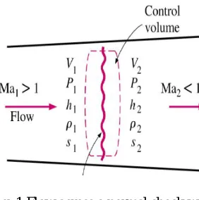
[image:2.612.233.374.505.647.2]

Normal shock: The portion of a shock wave which is perpendicular to the free stream is called the normal shock. Normal shock involved one dimensional flow in which the flow properties vary only with one coordinate direction.

Fig. 1 Flow across a normal shock wave

Stationary shock wave: a shock wave is stationary when the gas in which it propagates travels at the same speed equal to that of shock, but in opposite direction.

Technology (IJRASET)

The calculation of normal shock property on flow fields obviously requires thermodynamic and chemical relation which includes the real gas effects and the reactions and products. Anderson [1] carried out a simplified air model analysis, consisting of normal shock property calculation. The use of simplified air model enables us to show the basic features of hypersonic flow.

II. GOVERNINGEQUATIONS

Considering a rectangular control volume passing through the shock perpendicular to the flow, we can derive the continuity, momentum and energy equation. The fundamental flow equations, namely, the equation of continuity, momentum equation and energy equation can apply across a shock wave. Since there is an increase in entropy across the shock wave, the isentropic flow assumptions are not applicable, but changes assumed to take place adiabatically across the shock wave [2].

1 1

u

1 2

u







(1)

2 2

1 1 1

u

p

2 2 2

u

p











(2) 2 2 1 2 1 2

2

2

u

u

q

h







h



(3)

Equations are represented as continuity, momentum and energy equation respectively. Where q is the heat added per unit mass and

h e

 

pv

is, by definition enthalpy. Now in order to find out the properties behind the shock wave we make use of above equations.

In our research work has been confined to the solution procedures for the inviscid flow and the governing equations are known as the Euler equations. Euler equations are first order system of non-linear coupled equations, which can be expressed in various forms such as conservation form and primitive variable form. Conservation form of the equations is essential in order to compute correctly the propagation speed and the intensity of discontinuity, such as contact discontinuities or shocks that can occur in inviscid flows.

0

i i i

U F G

t x y

            (4) i i u U v E m                        2 i i u u p F uv uH um                         2 i i u uv

G v p

uH vm                        

The Euler equations governing the 2D flow [3] in the absence of body forces with species transport equation in the conservative and differential form are,

( ) ( ) ( )

0

u v

t x y

  

  

  

   (5)

2

( ) ( ) ( )

0

u u p v

t x y

  

   

  

   (6)

( ) ( ) ( )

0

E uH vH

t x y

  

  

  

   (7)

( ) ( ) ( )

0

i i i

m um vm

t x y

  

  

  

   (8)

Technology (IJRASET)

III.NUMERICALMETHOD

A. Finite Volume Method Formulation

The basic idea of a FVM is to satisfy the integral form of the conservation laws to some degree of approximation for each of many adjacent control volumes which cover the domain of interest.

V( ) ( )

. 0

t S t

d

UdV n Fds

dt









 

(9)

The average value of Uin a cell with volume V is

1

V

U



_

UdV

(10)

Eq. 3.1 can be written as

( )

. 0

S t

d

V U n Fds

dt 





  (11) ( ) 1 . 0 S t dU n Fds

dt V





 

(12)

U is the average value of U over the entire control volume, Fis the flux vector and n is the unit normal to the surface. AndFF i G jI  I

  

, is the total inviscid flux, upon integrating the inviscid flux over the faces of kth control volume the above equation becomes 1 1 . 0 nf k i k k U F nds

t V 

    _{ }   _



_   (13)

Here, i i

i i

y x

n i j

s s

 

 

 

  

and  si (x)i2 ( y)i2

For the 2-D axi-symmetric problems the finite volume formulation is given by

( ) 1 . 0 S t dU n Fds

dt V





 

(14)

B. Discretisation Schemes

In computational fluid dynamics discretisation of inviscid or convective fluxes is the critical part of Euler solver. One of the methods mentioned below is generally seen in the literature for computation of inviscid or convective fluxes-

Flux vector splitting scheme Flux difference splitting scheme

Total Variation Diminishing (TVD) scheme Fluctuation splitting scheme

In the present investigations Van-Leer scheme from the family of flux vector splitting schemes is preferred for present studies. The idea behind the flux vector splitting schemes is to divide the flux vector into positive and negative components.

C. Flux Vector Splitting Scheme

Technology (IJRASET)

developed by Steger J L [5] belongs to the second class of the Flux vector splitting scheme. Advantages of the Flux vector scheme includes with a little or moderate increase in numerical effort gives better resolution of shocks. Also this is well suited for implicit methods where the computation of steady state solution is of great importance. Main importance is that the Flux vector schemes can be easily extended to real gas flow.

D. Van-Leer Scheme

Van Leer flux vector splitting scheme is based on the characteristics decomposition of convective fluxes. He splits the convective flux in to positive and negative part based on the normal Mach number to the face of the control volume.

c _{c c}

F F F

 

  

, The Mach number normal to the face of the control volume is given by M_n u c



 ,Where

u

_is the contra variant

velocity, given by,

u

_



un

_x



vn

_yand c is the speed of the sound. The values of the flow variables



, ,

u v

and

p

are respectively have to be interpolated to the faces of the control volume. Then the positive fluxes are computed with left state and negative fluxes are computed with right state. The advection Mach number is given by

n L R

M MM Where the split mach numbers are defined as





2

if 1

1

1 if 1 4

0 if 1

L L

L L L

L

M M

M M M

M                    





2

0 if 1

1

1 , if 1 4

, if 1 R

R R R

R R

M

M M M

M M          _   _        

The mach numbers

M

_Land

M

_R are computed using the left and right state from the equation

L L L u M c   R R R u M c 

 , The normal flux vector is given by

x y u uu pn F vu pn Hu             _             

In the case of subsonic flow ( M <1) the positive and negative flux part are given by









( 2 ) /

2 /

mass mass x nor c

mass y nor energy

f

f u n u c F

f v n u c

f





                             

Technology (IJRASET)













2 2 2

2 2 2

2 ( 1) 4 1 4 1 2 2 2 1 L mass L L

R mass R R

nor _nor energy mass M f c M f c

u c u v u f f             _{     }      _  _     

For supersonic flow



M





1



fluxes are computed as

,

0 if

1

,

0 if

1

if -1<

1

F

F

F

M

F

F

F

M

F

F

F

M

                 











 







VanLeer flux vector splitting scheme performs very well in the case of Euler equations. But for viscous flow it smears out the boundary layer and also gives inaccurate stagnation and wall temperatures.

E. Boundary Conditions

In numerical simulation only a part of real physical domain is considered, this may lead to artificial boundaries were we need to specify the values of physical quantities To get an accurate numerical solution proper and correct implementation of boundary condition is necessary. Improper implementation of the boundary condition may lead to instabilities in the solution and lead to erroneous numerical result. Therefore one should give utmost care in selecting and implementing the boundary conditions. For 2-D inviscid flow problems the commonly encountered boundary conditions are

Inviscid or slip wall

Pressure extrapolation boundary condition Supersonic inlet and outlet

F. Evaluation Of Gradients

Gradients are needed not only for the constructing flow variables at the cell faces but also required for computing diffusion terms and velocity derivatives. The gradient



U

of a given variable

U

is used to discretises the convection and diffusion terms in the flow conservation equations. Gradients can be computed using the following methods

Green-Gauss Cell- Based Green-Gauss Node-Based Least Squares Cell-Based

G. Algorithm And Description About The Development Of In-House Solver

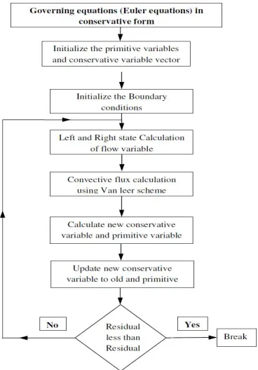
A brief description about the algorithm of solver is planning to discuss. The flow chart of the algorithm is as shown in Fig 2. Once the preprocessing is completed the primitive variables



, , . ,

u v T e

and conservative variables

 

,

u

,

 

v

,

e

are initialized in all cell centroids .Then the boundary conditions are initialized in the all boundary face centroids based upon the boundary type. Inlet boundary conditions are specified as same as that of free stream conditions. The outlet boundary conditions are extrapolated from the interior cell centroid. For inviscid wall boundary condition ghost cell approach is used for current solver. Intilization of the boundary condition is carried out by running loop over all the faces.

Technology (IJRASET)

flow variables at faces. Residuals are calculated from the relation



_{n1 n}



2

nc

 _

and it is being normalized by dividing the residual

[image:7.612.216.400.116.380.2]

calculated from the first iteration.

Fig. 2 Algorithm of the in-house solver

IV.RESULTANDDISCUSSION

The objective of this research paper is to discuss the results obtained from the present solver in comparison with the theories in hypersonic flow and with the standard Normal shock theory. Various test cases used to validate the code is planar flow past a cylinder. In this test case mentioned above the present solver results are validated across various theories in hypersonic flow theory.

A. 2-D Planar Flow Past A Cylinder

The inviscid flow past cylinder of radius 30 mm has been investigated for Mach numbers in the range 8.0. The fluid domain geometry and the corresponding mesh are shown in the Fig 3. The computational grid consists of 2000 cells. The important flow features of flow past a sphere consists of a bow shock wave detached from the body, which is a normal shock at the nose becoming weak downstream. Behind the normal portions of the shock wave flow is subsonic which during expansion becomes supersonic over the cylinder. Thus the flow in the shock layer is a mixed subsonic supersonic flow as seen in the typical Mach contour Fig 5. Also various contours have been seen via simulation for the better understanding of Normal shock. Since normal shock exists at the nose of the cylinder, property relations obtained from the solver has been compared with the normal shock relations [6] for





1.4

as shown in the Table 2.

B. Formulation Of Parameters

The following relations are to be used for calculation of property behind the normal shock.

2 2

1 1

2

1

(

1)

1

p

M

p





 





(15)

2 2

2 1

1 2

2 (

1)

2

[1

(

1)][

]

1

(

1)

T

M

M

T

M



















Technology (IJRASET)

2

2 1

2

1 1

(

1)

2 (

1)

M

M

















(17)

2 1 2

2

2 1

1

1 [(

)]

2

1

(

)

2

M

M

M

















[image:8.612.173.406.78.325.2]

(18)

[image:8.612.133.479.367.422.2]

Fig. 3 Computational domain for flow past cylinder

[image:8.612.137.475.445.706.2]

Table 1 Free stream condition for Cylinders

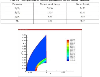
Table 2 Comparison of various parameters across shock (cylinder)

[image:9.612.186.425.74.619.2]

Technology (IJRASET)

Fig.5 Mach contours (M=8)

Fig. 6 Temperature Contour M=8 in Kelvin

Fig.7 Pressure Contour M=8 in Pascal.

V. CONCLUSION

Technology (IJRASET)

REFERENCES

[1] Anderson, J. D. (1989). Hypersonic and High Temperature Gas Dynamics. McGraw-Hill Inc. [2] Blazek, J. (2001). Computational Fluid Dynamics Principal and Applications. Eselvier.

[3] Venkatakrishnan V (1995), Convergence to steady state solutions of the Euler equations on Unstructured grids with Limiters, Journal of computational physics 118,120-13.

[4] Liou, M. S. and C. J. Steffen (1999). A New Flux Splitting Scheme. Journal of Computational Physics 107, 23-39.

[5] Steger J L and Warming R F (1981), Flux vector splitting of inviscid gas dynamic equations with application to Finite difference methods, Journal of computational physics, 40, pp 263-293.