Munich Personal RePEc Archive
Interest rate rule for the conduct of
monetary policy: analysis for Egypt
(1997:2007)
Rageh, Rania
Faculty of Economics and Political Science- Cairo University
8 May 2010
Online at https://mpra.ub.uni-muenchen.de/26639/
Interest Rate Rule for the Conduct of Monetary Policy:
Analysis for Egypt (1997:2007)
Working Paper Prepared By
Rania Rageh, PhD
Economist, Central Bank of Egypt
Abstract
ــــــــــــThis Working Paper should not be reported as representing the views of the CBE.
The views expressed in this Working Paper are those of the author(s) and do not necessarily represent those of the CBE or CBE policy. Working Papers describe research in progress by the author(s) and are published to elicit comments and to further debate.
The main objective of the paper in hand is to examine the validity of using Taylor rule as a robust rule for conducting monetary policy in case of Egypt. In this context, the paper
works through two main pillars. First: parts two and three; critically analyze the theoretical
grounds for using an interest rate rule in conducting monetary policy. Second: part four;
emphasize how the Taylor rule can be empirically estimated and evaluated. Consistently; this exercised while estimating and evaluating both simple backward and forward-looking Taylor rule for Egypt, guided by lessons from selected countries` experiences in estimating Taylor rule like U.S.A., U.K and Chile.
JEL Classification Numbers: E52; E58
Keywords: central bank, monetary policy, Taylor rule.
Contents Page
I. Introduction 4
II. Types of Monetary Policy Implementation 6
A- Monetary Policy-Rule based versus Discretion 6
B- The role of monetary policy rules in satisfying the goals of monetary policy 7
C- The central banks` reaction function 8
1- In case of closed economy 8
2- In case of open economy: The monetary policy reaction to the exchange rate 10
III. Taylor Rules: A Literature Survey 13
A- Taylor rule and its modifications 13
B- Uses and Abuses of the Taylor rule 16
C- Estimating the Taylor Rules 20
IV. Taylor Rule Applications: The Case of Egypt 22
A- Monetary policy in Egypt: historical review during 1990 to 2007 22
B- Constructing the model 31
1- The data 31
2- Methodology: the models 32
i- The first model: The central banks` reaction function 32
ii- The second model: The Augmented Taylor rule 40
V- Conclusion and Policy Implications 43
Tables
1: A Simple Matrix of Monetary Policy Reaction to the ExchangeRate 11
2: Data Description 32
3: The Interpretations of the Impulse Response Functions of the Open Economy
VAR Model 38
4: Augmented Taylor Rule Estimation Output Using GMM 40
5: The Illustrated GMM Output of the Augmented Taylor Rule 41
Figures
1: Discount Rate And 3-M T-bills Rate 24
2: Domestic Interest Rates 25
3: 3M Deposits Rate 26
4: Nominal Exchange Rate 29
5: Impulse Response Functions in Closed Economy 34
6: Variance Decomposition in Closed Economy 35
7: Impulse Response Functions in Open Economy 37
8: Variance Decomposition in Open Economy 39
References 45
Appendices
A: The Statistical Appendix 59
B: Estimating the Augmented Taylor as exercised in Part Four but with using the
I. Introduction
“The predominant weight of the existing evidence suggests that the effects of monetary policy on real economic activity are systematic, significant, and sizeable. Yet questions remain, both about individual empirical results and, more broadly, about the different methodological approaches that researchers have used to investigate these effects” Friedman (1995).
The quantity theory of money has overwhelmed the theory and practice of monetary policy for long, implying a long existing perception of monetary policy as a passive instrument in real economic activity, and central banks as merely institutional means of stabilizing monetary targets, denying the potential influence of central banks on real economic growth.
However, the increasing dominance of New Keynesian literature in recent decades subverts the orthodox view of monetary policy by building down the “Fisherian” assumptions on price and wage flexibility. The New Keynesian framework with prices or/ and wages rigidity, known as Dynamic Stochastic General Equilibrium (DSGE) Models, creates a channel for monetary policy to affect real macroeconomic variables through systematic policy actions using a monetary policy rule.
Although the significance of setting transparent policy rules through which central banks can manage market expectations was highlighted by Lucas and Sargent (1981). Nevertheless, the revival of academic and policy interest in “policy rules” was brought about with the introduction of John Taylor’s monetary policy reaction function known as “Taylor rule” in his famous "Discretion versus policy rules in practice" (1993), following closely the observed path of the U.S. short-term interest (Fed Fund rate) rate in the late 1980s through early 1990s. Taylor demonstrated that a simple reaction function (Taylor Rule) can respond to movements in fundamental variables (inflation and output gap) using a simple policy instrument (a short-term interest rate). Latterly, numerous modifications have been introduced to “Taylor’s Rule” (Clarida, Gali and Gertler, 2000; et al), with specific applications to the US economy and other countries.
Nevertheless, a particular gap in existent economic literature lies in disregarding the importance of studying the scope of applying monetary policy rules to various country groups; whether policy rules are fit for application in all countries or whether they are case-specific to certain economies, and if found adequately general for application in all central banks, what are the specified measures to adapting such rules to specific country cases.
interest rate rule was merely addressed in an implicit fashion, without explicit emphasis on both the theoretical rationale for using Taylor rule for monetary policy conduct, and how this rule can be empirically evaluated (Moursi, El Mossallamy and Zakareya, 2007). The thesis at hand is the first attempt to study these issues explicitly, whether theoretically or empirically. Hence, the purpose of this paper is to examine the validity of using an interest rate policy rule, specifically the Taylor rule, as a robust rule for conducting monetary policy in case of Egypt.
The time frame of the study at hand covers the period extending from January 1997 to December 2007 (on a monthly basis). This period experienced two key events for the
central bank of Egypt; first: floatation of the Egyptian pound at the end of January 2003.
The high inflation rates that came about in the aftermath of the floatation of the Egyptian pound seemingly encouraged the CBE to advocate price stability and low inflation rates
(along with banking system soundness) as the main monetary objective1. Second:
managing the short-term interest rate as an operational target for conducting the monetary
policy in June 20052, instead of excess reserves. This action was taken as a prerequisite
infrastructure for adapting an inflation-targeting regime, where the new system of policy management is based on conventional macroeconomic theorization, which predicts that it would be possible to stabilize output, prices and control inflationary pressures via monetary tightening. In practice, there are no assurances that the actual results obtained from a monetary contraction would match the theorized facts. In particular instances, an increase in interest rate could, in special circumstances, lead to a rise in the price and/or
output levels3.
Such mysteries are likely to expose the effectiveness of the CBE monetary policy and its capacity to check inflation and achieve the price stabilization objective. Consequently, an analytical need revealed for understanding the dynamic behavior of prices and output in response to different monetary policy shocks. Discerning the structure of those responses should also be useful to investigate the prospects of pursuing a monetary policymaking framework based on a formal inflation-targeting approach as proposed recently by the CBE (CBE 2004/2005).
1
The importance of realizing price stability as an intervening principal objective of monetary policy was further emphasized by the recent structural reforms, which encompassed the establishment of the Coordinating Council, under the leadership of the Prime Minister, in January 2005 and the Monetary Policy Committee affiliated to the CBE Board of Directors in mid-2005.
2
To manage the interest rates (including the overnight interbank rate) and implement its monetary policy, the CBE established a new operational framework early in June 2005, known as the corridor system, with a ceiling and a floor for the overnight interest rates on lending from and deposits at the CBE, respectively.
3
II. Types of Monetary Policy Implementation
Part two through three: the paper critically analyzes the theoretical ground for using and estimating an interest rate rule for conducting monetary policy. So, it begins with exploring the foundation of the interest rate rules and its monetary policy implementation alternatives. This is in addition to reviewing the advantages and disadvantages of each alternative.
The paper, then, highlights the role of the interest rate rules in satisfying the monetary policy goals. Finally, it discusses Taylor (2001) central bank reaction function in case of both closed and open economy, and the significance of the exchange rate in the open economy central bank reaction function.
A- Types of Monetary Policy Implementation: Rules versus Discretion
An extensive literature addresses the question of whether it is preferable to implement monetary policy by a rule or by discretion. This question has traditionally been referred to
as the issue of rules versus discretion (Federal Reserve Board, 2002).
In a strict interpretation of a rules-based regime; policymakers commit to how they will adjust their policy instrument, in response to incoming data or to changes in the forecast. Once this rule is specified, their judgment no longer is relevant to the policy outcomes. On the other side, in a discretionary regime, policymakers do not commit in advance to a specific course of action, but instead they apply their judgment, deciding on each occasion what policy is appropriate.
A strict rules-based policy establishes an unequivocal commitment by policymakers to achieve their policy objectives, especially meeting their inflation objective. Such a commitment, in turn, increases the transparency and accountability of monetary policy and thereby helps to pin down inflation expectations. In principle, the resulting credibility about policymakers' commitment to price stability could reduce the cost of disinflation, if inflation were to rise above the objective, and could reduce the spillover of supply shocks-that is autonomous shocks to the price level-into broader price movements.
In this spirit, in 1993, John Taylor a systematic monetary policy informed by policy rules but flexible enough to adapt to structural changes and other real-world complexities. This was in many economists` view, the best direction for monetary policy. This regime based on complementarity between rules and discretion was encouraged by John Taylor was widely discussed. It provides the advantage of the both the rules based and discretionary monetary policy, where it shows that the usage of the rules should be as a good guidance to policymakers which could improve their judgmental adjustments to policy.
B- The role of monetary policy rules in satisfying the goals of monetary policy
The time inconsistency literature argues4 that a purely discretionary policy setting leads to
higher long-run inflation (Kydland and Prescott 1977, and Barro and Gordon 1983). In
such circumstances, a credible commitment by the central bank to maintain price stability can reduce the inflation bias from monetary policy. In the past, such a commitment was often imposed externally by a fixed exchange rate, or internally by a monetary growth target. However, in the meantime, both approaches have lost their importance: the former has proved to be unsustainable in the face of growing capital flows and financial markets’ imperfections, and the latter has failed because of large-scale shocks to money demand functions.
Against this backdrop, a recent and growing body of literature has argued that inflation targeting provides a convenient mechanism for central banks to combine rules and discretion in conducting monetary policy. For example, Svensson (1999) describes inflation targeting as “decision making under discretion” where central banks follow what he calls a “targeting rule” by which they set interest rates to reduce the deviation between the conditional inflation forecast (the “intermediate target” of policy) and the inflation
target to zero over the target horizon5. In this setting, the central bank is not committed to
any particular instrument arrangement and therefore gains considerable flexibility in setting its interest rate. The typical process involves the central bank revising its inflation and output forecast in each period (corresponding to the frequency of the monetary policy committee meetings) based on the information available to it at that time. If the conditional inflation forecast is higher than the target, the central bank will increase the interest rate to minimize such deviations by the end of the targeting horizon, and vice versa. The private sector then decides its consumption and investment plans based on the central bank’s reaction. Blinder (1998) calls this “enlightened discretion” and argues that it is close to
what many policymakers try to do in practice6.
4
As discussed in the above section.
5
Similarly, Bernanke and Mishkin (1997) characterize inflation targeting as a framework under which policymakers exercise “constrained discretion”. According to White (2002), an important practical benefit of rules in monetary policy is that they can constrain the behavior of central banks and promote transparency.
6
The need for greater monetary discipline in emerging market economies has been generally stressed against the backdrop of their relatively high inflation and low policy credibility. In a recent paper Calvo and Mishkin (2003) discuss why emerging market economies are vulnerable to “sudden stops” of capital inflows and repeated exchange rate collapses. Attributing financial crises in emerging market economies to their weak institutional credibility, they suggest that central banks in these economies should be subject to “constrained discretion” through inflation targeting, making it harder for them to follow an “overly expansionary monetary policy”. To the extent that this leads to a more transparent and accountable instrument setting behavior by the central bank, it can pin down investors’ confidence and reduce vulnerability to crisis.
Taylor (2002) provides another reason for adopting a rule-based monetary policy in emerging economies. He argues that anticipation effects of monetary policy are higher when the central bank follows a systematic approach in setting interest rates. Given their less developed financial markets, such effects are likely to be lower in emerging economies. Yet monetary policy could still have significant impacts through movements of wages and property prices. More predictable central bank behavior is therefore expected to improve the transmission and effectiveness of monetary policy. Indeed, over the last
decade of the 20th. century, the conduct of monetary policy in emerging market economies
has increasingly moved in this direction.
C- The central banks` reaction function:
Given the above discussion, there are reasons to believe that central banks’ reaction function-especially in emerging market economies-needs to consider their multiple objective setting.
The equations stated below summarize the standard aggregate model where the central bank sets the interest rate according to both the inflation and the output gap as follows (Taylor 1999):
1- In case of closed economy:
……… (1) ………….... (2) ……….(3)
Equations (1) and (2) are the closed economy aggregate demand and supply equations (backward-looking Phillips curve).
Equation (3): defines the policy rule, whereby the central bank changes its policy rate
according to the current period inflationary and output gap, given the policy parameters δ0,
δ1, and δ2.
A crucial condition for the stability of this model is that the reaction coefficient on inflation
(δ1) should be above unity
7
. The aggregate demand function is then negatively sloped with respect to the inflation rate. Faced with a price shock (e) the central bank increases its interest rate by more than the rise in inflation, which raises real interest rates until inflation returns to the target.
Given the underlying Phillips curve relationship in (2), the coefficient on the output gap
(δ2) in the reaction function depends on two factors: the slope of the aggregate supply
curve and the weight given to the variability of output in the loss function. For instance, a flat supply curve implies that a policy shock to reduce inflation will significantly increase output variability, suggesting, ceteris paribus, a relatively small coefficient.
Moreover, a standard practice followed by many researchers is to include a lagged interest rate term in the reaction function (3), reflecting the desire of central banks to smooth interest rate changes. The economic rationale behind such smoothing has been well
documented in the literature8. Moving the policy rate by small steps in the same direction
increases its impact on the long-term interest rate because market participants expect the change to continue and hence price their expectations into forward rates. Acting gradually also reduces the risk of policy mistakes, when uncertainty about model parameters is high and policymakers have to act on partial information.
Another reason is that central banks may care about the implications of their actions for the financial system: if markets have limited capacity to hedge interest rate risk, a sudden and large change in the interest rate could expose market participants to capital losses and might raise systemic financial risks.
Other reasons could include avoiding reputation risks to central banks from sudden reversals of interest rate directions.
7
Substituting equation (3) into equation (1) gives the slope of the aggregate demand function as -β(δ1 - 1)/(1+ βδ2). Hence the stability of the policy rule requires that δ1 >1.
8
2- In case of open economy: The monetary policy reaction to the exchange rate
The exchange rate is the key variable while speaking about the monetary policy reaction function in the context of open economies. Particularly, when the exchange rate pass-through into prices is very high, this key variable is likely to assume a special importance for the monetary policy.
Focusing upon an open economy interest rate reaction function, the central bank reacts to the actual inflation rate, output gap, and the changes in the exchange rate in the following way (Taylor (2001):
……… (1) ………….... (2) ………. (4)
where: y, i, π, xr and r are the output gap, the central bank policy rate, the inflation rate, the log level of the real effective exchange rate, and the long-run equilibrium real interest rate respectively. β, α, δ are slope parameters and u & e are stochastic disturbance terms. ∆ is the first difference operator.
Reasons behind adding the exchange rate to the interest rate reaction function in case of open economy:
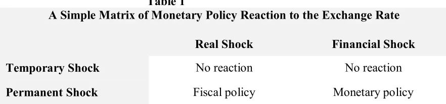
A familiar argument, pioneered by Taylor (2001), is that if the exchange rate depreciates due to a temporary disturbance, the interest rate should remain unchanged (first row of Table A below). This is because such exchange rate movements do not have much effect on expectations of inflation, and a central bank that reacts to inflation will indirectly take
into account the consequences of the exchange rate movement for its policy9. If the
depreciation is due to a decline in the demand for exports, the central bank faces a positive price shock as well as a negative demand shock, making an interest rate increase less necessary.
Attempts to reduce exchange rate volatility might also increase output volatility; Ball (1999) shows that, in such circumstances, targeting a long-run inflation rate that excludes exchange rate effects is more helpful. This may increase the short-run inflation volatility, but will greatly reduce output variability.
9
Mishkin and Savastano (2001) argue that reacting “too heavily and frequently” to exchange rate movements raises the risk that the exchange rate might become the de facto anchor for monetary policy.
Table 1
A Simple Matrix of Monetary Policy Reaction to the Exchange Rate
Real Shock Financial Shock
Temporary Shock No reaction No reaction
Permanent Shock Fiscal policy Monetary policy
Source: derived by the author.
Another case theoretically meriting no monetary response, is a depreciation caused by a permanent real shock; for instance, a secular decline in the terms-of-trade or a negative productivity shock. A first best policy may be to adjust other policies, in particular fiscal policy to align the aggregate absorption level in the economy (second row of Table A, left-hand column).
On the other hand, Ball (2002) points out that if the adverse exchange rate shock is from the financial side (for example, a sudden withdrawal of foreign investors from the country), an increase in the interest rate may be an appropriate response to stabilize both inflation and output (second row of Table A, right-hand column). While currency depreciation will increase external demand and prices, a higher interest rate will reduce domestic demand
and stabilize inflation10.
Nevertheless, in practice, many emerging market economies intervene to stabilize the exchange rate by changing interest rates, and the scale of such intervention also tends to be large. This raises the question of the factors that may account for this behavior. One reason, consistent with theory, is that major currency depreciations in emerging market economies have, in fact, been due to financial shocks, often resulting in high inflation. Second, exchange rate shocks tend to be large and persistent in emerging economies, which can create a dilemma for the central bank. If it chooses to absorb the exchange rate depreciation it might risk overshooting the inflation target and lose credibility. At the same time, defending the currency might require raising the interest rate to a very high level, which can cause large output losses.
10
In a recent study, Ho and McCauley (2003) show that emerging economies that miss their inflation targets are generally the ones experiencing sharp exchange rate volatility. This suggests that central banks may be ready to raise rates when faced with large currency depreciations. But they may, at the same time, prevent sharp contraction of the economy even at the cost of missing the inflation target.
Central banks in emerging market economies may also assign a relatively higher weight to the exchange rate for reasons other than price stability - most importantly, maintaining financial stability.
Calvo and Reinhart (2002) attribute such “fear of floating” behavior on the part of emerging economies to the high risk premium they have to pay because of their low
institutional and policy credibility11. Such resistance to floating may be particularly high in
countries with thin exchange markets, which are vulnerable to one-way expectations and herd behavior. A disorderly depreciation can encourage speculation through leads and lags in trade transactions and short-term capital flows, giving the exchange rate its own momentum.
Many recent experiences of exchange market intervention go to support this concern. Partly because its exchange market is thin, India has tried to avoid excessive exchange rate volatility through foreign-exchange and interest rate interventions. When the Philippine peso came under strong depreciation pressure in the middle of 2001 and again in early 2003, the central bank raised reserve requirements to limit currency speculation (Mohanty and Klau 2004).
In some cases, financial imperfections such as a large amount of external debt or debt indexed to the exchange rate may have made the case for monetary policy intervention even stronger. Eichengreen (2002) and Goldstein and Turner (2004) have recently highlighted the adverse consequences of exchange rate depreciations in countries with a high degree of dollarization. Sharp currency depreciations in such circumstances, it is argued, can cause widespread bankruptcies and even change the sign of the exchange rate in the aggregate demand function from positive to negative.
This rather unconventional contractionary impact of the exchange rate makes it necessary
for the central bank to raise rates defensively against major exchange rate shocks12.
11
In a recent paper, Alesina and Wagner (2003) argue that the “fear of floating” critically depends on the state of political institutions. Countries with poor political institutions end up with more volatile exchange rates than countries with sound political institutions.
12
III. The Taylor rule:
A Literature Survey
After exploring the foundation of the interest rate rules and its monetary policy implementation alternatives in the previous section, the paper focuses on the initial interest rate rule “Taylor (1993)” and its modifications ending with showing the augmented Taylor rule which is tailored for each individual country case. The paper, then, highlights how the interest rate rules can be used or abused while implementing monetary policy, from both descriptive and perspective points of view. In addition; it discusses both foundations of the theoretical and empirical choice of a benchmark rule
Finally, after the previous theoretical base, the paper sheds light on how Taylor rule can be statically estimated and the best way to interpret and implement it.
A- Taylor rule and its modifications
Taylor Rule (1993) defined as; a simple rule works through an instrument13, which
responds only to both inflation and output gap.
Taylor (1993) suggested this rule as an explanation of the monetary policy setting for the early years of Alan Greenspan’s chairmanship of the Board of Governors of the U.S. Federal Reserve System, thereafter “the Fed” (1987–92). This rule became very popular, since it described a complicated process in very simple terms and fitted the data very well.
Starting by a description for the original Taylor rule (1993) and present the modifications it has since undergone:
- The Taylor rule (1993):
……….. (5)
where: it is the short-term nominal interest rate in period t; r* is the real interest rate; πt- π* is the “inflation gap” which represents the difference between the actual inflation πt and the inflation target π*; yt = log Yt – log Y*t is the output gap, where Yt is the real GDP and Y*t is the potential output14, and the coefficients Cπ and Cy are positive.
In the original Taylor (1993) formulation, Cπ and Cy were both 0.5, the inflation and real
interest rate targets were 2 percent each, and hence the constant C was equal to 1.
13
The policy rate (the nominal short-term interest rate).
14
Taylor (1993) identified potential output empirically with a linear trend, while other papers use quadratic, Hodrick-Prescott trends, or other more sophisticated techniques.
t y t t
y t
t
t r C C y C C C y
This original Taylor rule has undergone various modifications as researchers have tried to make it either more realistic or appropriate. This part will discuss those modifications
suited for rules not based on asset prices15, since these are the ones most commonly used.
• One modification to the original rule has been to incorporate forward-looking behavior in order to counteract the seeming shortsightedness of policymakers, making the short-term interest rate a function of central bank expectations of output gap and inflation rather than
their contemporaneous values16.
• An alternative modification has been to introduce lags of inflation and output gap. It has been pointed out in the literature that because it is not possible to know the actual output gap and inflation at the time of setting the interest rate, using lags would make the timing
more realistic (McCallum, 1999a)17.
• Interest rate-smoothing behavior (including a lagged short-term interest rate among the fundamentals) is the single most popular modification of the Taylor rule. Clarida, Gali, and Gertler (1999) note that, although the necessity of including an interest rate smoothing term has not yet been proven theoretically, but it seems rather intuitive for several
reasons18.
• As simple as it is, the Taylor rule cannot possibly take into account all the factors affecting the economy. Policymakers are known to react not only to movements in the output gap and inflation, but also to movements in the exchange rate, stock market, and political developments, etc. The way to capture this issue would be to introduce a new variable, a so called policy shock variable, reflecting the judgmental element of the policymaking process.
• Some authors suggest the use of unemployment gap as opposed to output gap, to improve the fit of the data, as suggested by Taylor (1999) and Orphanides and Williams (2003).
• This modification reflects Okun's law (1962), which links the output gap and the unemployment gap. This type of rule tends to perform quite well in terms of stabilizing
15
For estimations of monetary policy rules with asset prices and exchange rates in industrial countries, see Chadha, Sarno, and Valente (2004).
16
The central bank expectations considered are either formed within a model, as in Clarida, Gali, and Gertler (2000), or actual estimates of the central bank in real time, as done by Orphanides (2001). Mehra (1999) has estimated short-term interest rate as a function of inflation expectations contained in bond rates.
17
Lag-based rules are not necessarily backward-looking, since lags serve as indicators of future values (see Tchaidze, 2004).
18
economic fluctuations, at least when natural rates of interest and unemployment are
accurately measured19.
• Finally, it has been suggested to use rates of growth of unemployment, or of the output gap, to account for measurement errors in the real-time estimates of the natural rate of unemployment and/or output (McCallum, 1999a, and Orphanides and Williams, 2003).
So; many modifications have been made to the simple Taylor rule equation(5) (as Orphanides, 2001; etc.), to include more other variables as the exchange rate and the lagged nominal interest rate.
These modifications were made according to each individual country case, using the variables which could affect the country’s monetary policy reaction function most as shown in the next equation:
…….. (6)
where: it is the short-term nominal interest rate in period t; r* is the real interest rate; πt- π* is the “inflation gap” which represents the difference between the actual inflation πt and the inflation target π*; yt is the actual output and y*t is the potential output, xr is the log level of the real effective exchange rate, and ∆ is the first difference operator. γ1, γ2, γ3, γ4, γ5 are the policy parameters, and εt is the stochastic innovation.
Equation (6) usually referred to as the Augmented Taylor Rule; where it is tailored for each individual country case.
19
The rules with the unemployment gap appear more attractive as the natural rate of unemployment seemed easier to measure. During the mid–1990s, it was a common belief that NAIRU was 6 percent flat. The productivity growth of the late 1990s and arrival of the so-called New Economy have begun, only with a substantial delay, to challenge this belief (see Ball and Tchaidze, 2002).
t t t
t t
t t
t
t r y y xr xr i
i = +π +γ π −π +γ − +γ3∆ +γ4∆ −1+γ5 −1+ε *
2 *
1( ) ( )
B- Uses and Abuses of the Taylor rule
Taylor rules have been widely used in theoretical and empirical papers, with the latter examining the rules both from descriptive and prescriptive points of view.
The focus of research in theoretical papers has been on: whether simple rules solve the time inconsistency bias (McCallum, 1999a); or they are optimal (McCallum, 1999a;
Svensson, 2003; Woodford, 2001; etc.)20; and on how they perform in different
macroeconomic models (Taylor, 1999; Isard, Laxton and Eliasson, 1999)21.
As for the empirical papers, those with a descriptive point of view include analysis of
various specifications and estimations of the Taylor rule (Clarida, Gali and Gertler, 1998; Kozicki, 1999; Judd and Rudebusch 1998; etc.). These studies examine particular historical episodes and address two questions: to what extent are simple instrument rules good empirical descriptions of central bank behavior; and what is the average response of
the policy instrument to movements in various fundamentals?22
Empirical papers with a prescriptive point of view suggest what the interest rate should be
(McCallum, 1999a and 1999b; Bryant, Hooper, and Mann, 1993; Taylor, 1999), or how it should be set. Commonly, these suggestions are based on rules that are either the outcome of theoretical papers or the result of estimating “good/successful” periods of monetary policy.
The potential abuses in prescriptive papers are mainly related to the choice of the
benchmark rules, whether based on theory or empirical evidence. The following part provides a brief description of the problems that might arise when choosing such rules.
20 One could derive versions of the Taylor rule as a solution to an optimization problem, where policymakers are minimizing a loss function expressed in terms of the weighted average of inflation and output gap variances (see for example, Woodford, 2001).
21
In terms of stabilizing inflation around an inflation target, without causing unnecessary output gap variability.
22
Theoretical Choice of a Benchmark Rule Policy: advice based on rules from theoretical models comes from rules simulated or derived in a model or class of models considered representative of the economy. There are potential problems with this approach as documented in the literature and surveyed below:
• Svensson (2003) and Woodford (2001) warn that commitment to simple rules may not always be optimal, as a simple policy rule may be a solution too simple for a task as
complex as that of a central bank23.
• Simple policy rules may not be robust across different models. Due to uncertainty about the true model of the economy and/or potential output levels, the most recent theoretical efforts have concentrated on suggesting a set of robust simple rules that could be used as a basis for policy advice, as in Giannoni and Woodford (2003a and 2003b), Svensson and Woodford (2004), Walsh (2004), etc. Isard, Laxton and Eliasson (1999) show that several classes of Taylor type rules perform very poorly in moderately nonlinear models.
• Several recent papers show that, when the central bank follows Taylor type rules in sticky price models of the type that fit the U.S. data well, the price level may not be determined, and there could be several paths for the instrument and multiple equilibria, all coming from the same model with the same rule (Benhabib, Schmitt-Grohe, and Uribe, 2001; Carlstrom and Fuerst, 2001; etc.).
• How policymakers should respond to the presence of measurement errors is a question with no firm answer yet. While some researchers advocate a more cautious approach, with smaller response coefficients (Orphanides, 2001), others advocate a more aggressive approach (i.e., with larger coefficients) to policymaking (Onatski and Stock, 2002). Finally, some studies have argued in favor of “certainty equivalence,” which implies no changes in policymakers’ behavior and response coefficients (Swanson, 2004).
• Most theoretical papers talk about inflation in rather generic terms. Thus, when it comes
to policy prescriptions, it is not clear what particular measure should be used − Consumer
Price Index (CPI), core CPI, CPI less food and energy (most volatile items), GDP deflator, etc.
• Even after a particular index is chosen, there are more choices to make: annual or quarterly; if annual, is it the average of quarterly numbers or a growth rate over the four quarters? Is the growth in CPI calculated as a log difference or a ratio? Even though the
23
differences between these various calculations could be minimal in a case of low and stable inflation, one should be aware of these caveats. Similar issues arise when it comes to measuring the output gap.
• Any formula-based recommendation is bound to ignore the judgmental element, which reflects policymakers’ account of other developments not reflected in the output gap or inflation behavior.
Empirical Choice of a Benchmark Rule: Policy advice based on rules from empirical
papers comes, usually, from estimating a period that is considered “good” or “successful” in combating inflation, promoting output growth, or both. Like the theoretical approach this empirical approach brings with it several problems:
• Rogoff (2003) notes that, it is not clear how much credit policymakers deserve for the exceptionally good performance of many economies in the last 15 years or so. He notes that the achievement of price stability globally may be due not only to good policymaking but also to the favorable macroeconomic environment. The main cause that he identifies is globalization, which through increased competition, has put a downward pressure on prices.
• Stock and Watson (2003) also argue that improvements in the conduct of monetary policy after 1979 are only partially responsible for reducing the variance of output during business cycle fluctuations. This could have been caused by “improved ability of individuals and firms to smooth shocks because of innovation and deregulation in financial markets” (Stock and Watson, 2003, p. 46). They also note that during this period, macroeconomic shocks were “unusually quiescent”.
• Even if one finds empirically a Taylor rule, it does not imply that it is the basis of the monetary policy decision making. The empirical relationship found may be a reflection of something else – a long-term relationship among the nominal interest rate, inflation, and
the output gap24, or a reflection of a completely different kind of monetary policy25.
• Also as Svensson and Woodford (2004, p. 24) note, “Any policy rule implies a ‘reaction function,’ that specifies the central bank’s instrument as a function of predetermined endogenous or exogenous variables observable to the central bank at the time that it sets
24
As the definition of the rule (see equation (5)) shows, one may view the Taylor rule as a more sophisticated version of an equilibrium relationship among the three variables (also known as a Fisher equation, i = r + π).
25
the instrument.” They warn that this “implied reaction function” should not, in general, be confused with the policy rule itself.
• When making policy prescriptions, can one really impose the implied response coefficients and targets of one economic or policy regime on another, without accounting for changes in the structure of the economy? Greenspan particularly has warned about this abuse on several occasions, including in January 2004 in his speech to the American Economic Association (AEA) meetings: “Such rules suffer from much of the same fixed-coefficient difficulties we have with our large-scale models.”
• Even though there may be no changes in the economy, there may be changes in the attitude of policymakers. Such changes could be reflected in a shifting of targets for real interest rate or inflation (which, in terms of Taylor rules, translate into a different constant), or there may be changes in the weights that policymakers assign to inflation variance and output gap variance (which, in terms of Taylor rules, translates into different inflation and output gap response coefficients).
• Coefficients might not be estimated with a very high degree of precision, and standard errors could be quite large. Once the size of the confidence intervals is taken into account, the policy recommendations on how the instrument should be set could become blurred.
• While coefficients may be estimated for very particular measures of inflation and/or the output gap (for example, CPI less food and energy and Hodrick-Prescott (HP) detrended log output), it is the values only that get “remembered”, when policy recommendations are made. These coefficients may be coupled with different measures (for example, GDP deflator and linearly detrended log output, which in general results in larger values for the output gap than the HP detrending), without taking into account that the coefficients would have been different, in the sense that, these alternative measures been used for the estimation.
C- Estimating Taylor Rules
The rules are usually estimated using either ordinary least squares (OLS), if they are backward looking (see, for example, Orphanides, 2001), or instrumental variables and generalized method of moments (GMM) if they are forward looking (see, for example, Clarida, Gali, and Gertler, 2000), and it is not obvious that the following econometric problems are addressed properly, or always taken into consideration:
• The most obvious econometric question is how to deal with high serial correlation of the variables. The common recipe is to use Newey-West standard errors and serial correlation robust estimators in order to account for heteroschedasticity, and instrumental variables to account for the forward-looking rules. What is worth noting, however, is that while papers estimating Taylor rules commonly treat interest rates as stationary series, most term
structure and money demand papers treat interest rates of various maturity as I(1) series26,
which would call for different econometric techniques.
• The estimates are not very robust to differences in assumptions or estimation techniques. Jondeau, Le Bihan, and Galles (2004) show that, over the baseline period 1979–2000,
alternative estimates of the Fed’s reaction function using several GMM estimators27 and a
maximum likelihood estimator yield substantially different parameter estimates. Estimation results may also not be robust with respect to sample periods, to different sets of instrumental variables, or to the order of lags (when lags of variables are used as instruments).
• In addition, estimation of the Taylor rules very often requires inputs from separate estimation exercises, such as an evaluation of the output gap. These procedures are subject to the same kinds of problems, and, hence, the level of uncertainty around coefficients doubles.
• As in other empirical papers, making policy recommendations based on rules estimated from a short sample is not advised. This caveat applies especially to countries that have short periods of stable data.
• The alternative use of long samples often ignores the possibility of changes in the parameters of the rule—response coefficients or real interest rate or inflation targets. For
26
King and Kurmann (2002) analyze the term structure of the U.S. interest rates, and Baba, Hendry, and Starr (1992) analyze the U.S. money demand. Both papers find that U.S. interest rates are stationary in first differences, and therefore non-stationary in levels, I(1) series. However, Mehra (1993) finds in money demand studies that U.S. interest rates are stationary series, and Clarida, Gali, and Gertler (2000, p. 154) note that they treat interest rates as stationary series, “an assumption that we view as reasonable for the postwar U.S., even though the null of a unit root in either variables is often hard to reject.”
27
example, one should make a distinction between the monetary regime of the Fed during Paul Volcker’s chairmanship and that during Greenspan’s chairmanship. While, in both periods, the Fed was committed to price stability, it is doubtful that inflation targets were
the same28. A former Fed Governor, Janet Yellen (Federal Reserve Board, 1995, pp. 43–4),
confirms this implicitly when she says that the Taylor rule seems to be a good description of the Fed’s behavior since 1986, but not of its behavior from 1979 when Volcker was
appointed chairman, to 198629.
• A rather important but still commonly overlooked caveat has been given by
Orphanides (2001, p. 964). He finds that real-time policy recommendations differ considerably from those obtained with ex-post revised data, and that estimated policy reaction functions based on such data provide misleading descriptions of historical policy
and obscure the behavior suggested by information available to the Fed in real time30.
• The illusionary effects of a stronger or weaker response to movements in certain fundamentals that arise due to their horizon misspecification are documented by Orphanides (2001). It showed that the policy reaction function, which has forward-looking behavior but includes forecasts of less than four quarters ahead, has higher estimates for the lag of the federal funds rate and for the output gap, but lower estimate for inflation, compared with the specification with forecasts of four quarters ahead.
• Another illusionary effect, which is caused by monetary policy inertia, is documented by Rudebusch (2002). He argues that a policy rule with interest rate smoothing is difficult to
distinguish from a rule with serially correlated policy shocks31. While in the former
persistent deviations from the output gap and inflation response occur because policymakers are deliberately slow to react, in the latter these deviations reflect policymakers’ response to other persistent influences. Rudebusch proposes to distinguish between the two by analyzing the interest rate term structure.
Finally; economists should carefully estimate Taylor rules in practice, taking into consideration the above issues, otherwise they will end up with misleading results.
28
In fact, one may wonder whether the Fed had a constant inflation target during Volcker’s chairmanship (see Tchaidze, 2004).
29
“It seems to me that a reaction function in which the real funds rate changes by roughly equal amounts in response to deviations of inflation from a target of 2 percent and to deviations of actual from potential output describes tolerably well what this Committee has done since 1986.’’(Federal Reserve Board, 1995 p. 43---4).
30
Orphanides (2003a) shows, contrary to other researchers who claim that U.S. monetary policy in the 1970s was "bad," leading to high inflation, that policy was "good" but based on "bad," misleading data.
31
IV. Taylor Rule Applications:
The Case of Egypt
In this section; the entire theoretical basis previously discussed are considered while estimating the Taylor Rule in case of Egypt.
During the study period, Egypt switched between different regimes while implementing both monetary and the exchange rate policies, so the starting point will be reviewing Egypt’s monetary policy historical background. This guides the paper through both building up and interpreting the model.
The paper, then, estimates both the central bank reaction function and the augmented Taylor rule models using the E-views econometric package, and interprets the output.
Thus, this section will be presented as follows:
A- Monetary policy in Egypt: An overview during 1990 to 2007
B- Constructing the model
1- The data
2- Methodology: the models
i- The first model: The central banks` reaction function
ii- The second model: The Augmented Taylor rule
A- Monetary policy in Egypt: an overview during 1990 to 2007
This section presents a brief historical review for the main components of the Central Bank of Egypt’s monetary policy framework. The review considers the recent developments in the ultimate objective of the CBE monetary policy, the intermediate and operational targets that were selected to achieve that objective and the monetary instruments adopted to affect those targets. In addition, the paper reviews the exchange rate developments. In this context, we divide Egypt’s` monetary policy framework into three components:
• First: the ultimate (principle) target of the monetary policy
During 1990 through 2003, with the exception of 1996/1997, the CBE has continually focused on achieving two main objectives, namely, price stability and exchange rate stability. The monetary policy, however, exhibited overt inconsistencies, particularly during 1992/1993-1996/1997. In 1992/1993, besides price and exchange rate stability, the CBE planned to achieve ostensibly conflicting objectives; while the CBE aimed at
controlling the monetary expansion through implying a contractionary policy, it also called
for a cut of the interest rate on the Egyptian pound to encourage investment and promote
At the second stage of the economic reform program 1993/1994, the thrust of the monetary policy shifted to the promotion of growth in the productive sectors as a means of stimulating aggregate productivity (CBE 1993/1994). The CBE primary objective shifted back to the expansionary monetary control and output growth recipe during the 2-year period 1994/1995 to 1995/1996. In 1996/1997, the CBE reverted once more to the objective of economic growth via monetary stabilization.
In 2003 and going forward ,the CBE announced it ultimate target to be price stability, stated by the Law 88 for year 2003 regarding the central bank, the banking sector and foreign exchange.
• Second: CBE intermediate and operational targets
Alternatively, throughout the period 1990/1991 until 2004/2007, the different proximate targets of monetary policy seemed fairly consistent. The CBE intermediate target entailed the control of the annual growth rate of domestic liquidity measured in terms of the broad money supply, M2. Similarly, during the entire period under consideration, save 2004/2005, the two operational target components, management of nominal interest rates and the control of banks' excess reserves in domestic currency at the CBE, remained unchanged. Starting from June 2005; the overnight interest rate on interbank transactions was designated as the operational target.
• Third: CBE monetary policy instruments
To achieve its targets, the CBE depended mostly on a number of indirect, market-based instruments such as the required reserve ratio, reserve money and open market operations along with a host of interest rates including the discount rate, Treasury-bill rate, and loan and deposit interest rates. The choice of indirect instead of direct instruments was motivated by the initiation of the monetary policy reform act as part of the country's overall economic reform program signed with the IMF.
* Direct instruments: (e.g., quantitative and administrative determination of interest rates
* Indirect instruments (where the CBE started to exercise since 1991 with the advice of the IMF, under the structural reform program):
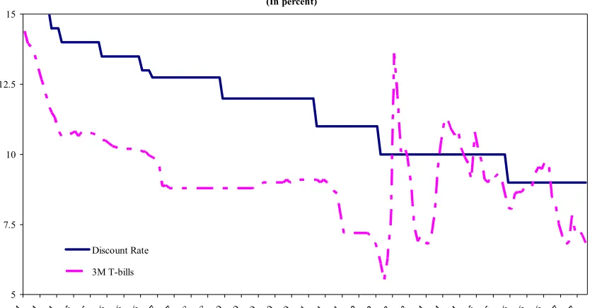
- The discount rate: the CBE use the discount rate as a monetary policy instrument during 1990 to 2007. During that period, the discount rate was lowered gradually from 19.8 percent in 1992 to approximately 9 percent by the beginning of 2006 and continue to hold
tell the end of 2007, with the hope of promoting investment32.
To reduce the rigidity in the discount rate, the CBE linked it to the interest rate on Treasury Bills. This resulted in a steady decline in the interest rate on Treasury Bills, which decreased starting 1992 through 1998 (See Figure 1). The interest rate on Treasury Bills began to recover once again in 2002 only to attain a maximum in the following year.
Source: CBE data.
32
[image:25.612.91.508.291.509.2]The discount rate is typically considered a poor operational monetary policy instrument because it is usually subjected to strong administrative control. Thus, shocks in the discount rate do not always account for variation in the monetary stance (Bernanke and Mihov 1998). In Egypt; the discount rate characterized with rigidity, where it used to held unchanged for long periods. Rageh (2005)
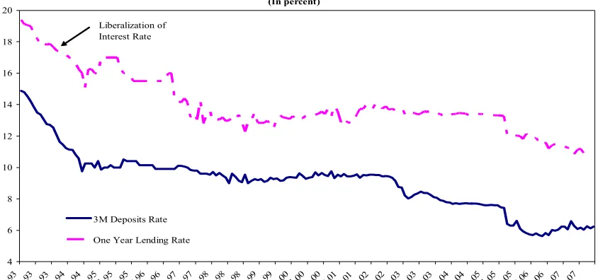
- The interest rates on loans and on deposits: by January 1991; the CBE had liberalized the interest rates on loans and on deposits. Banks were given the freedom to set their loan and deposit interest rates subject to the restriction that the 3-month interest rate on deposits should not fall below 12 percent per annum. This restriction was cancelled thereafter in 1993/1994 (See figure 2).
Source: CBE data.
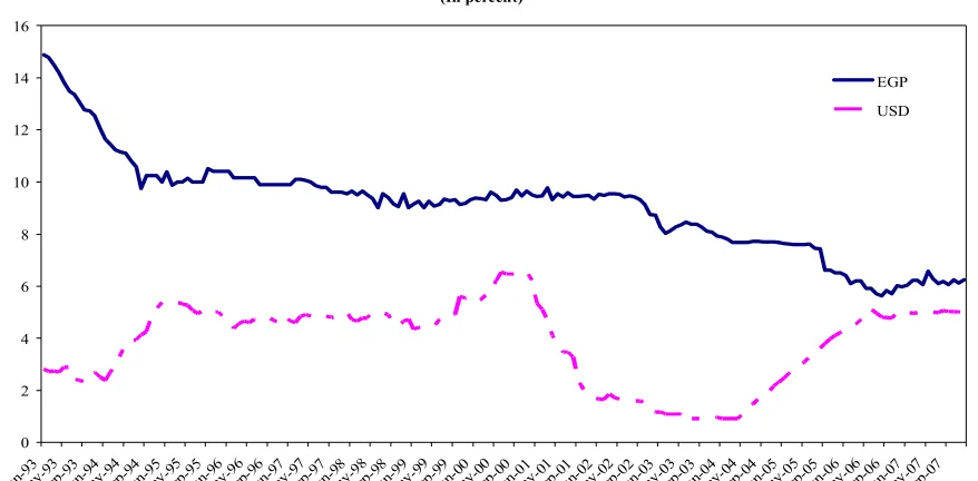
- Due to the continuous decrease in the discount rate, interest rates on loans (one year or less) also fell during the period 1995-1999 before they started to rise slightly again in 2000. The decline in the interest rate on loans led to a reduction in the returns on deposits held in domestic currency. The domestic currency deposits, however, were not significantly affected by the fall in the interest rate since the interest rate on the Egyptian pound deposits
remained relatively higher than the equivalent rates paid on foreign currencies33 (See figure
3) (El-Asrag 2003).
33
[image:26.612.94.521.181.379.2]Showing a 5 percent average spread on the 3-month EGP-USD deposit rates during the period 1995-99, derived from CBE data.
Figure 2: Domestic Interest Rates (In percent) 4 6 8 10 12 14 16 18 20 Ja n-93 Jun-9 3 Nov -9
3 Apr-94Sep -9
4 Feb
-95 Jul-95De
c-95 May -9
6 Oct
-96 Ma
r -97 Aug
-97 Jan-98Jun
-98 Nov -9
8 Apr-9 9 Sep-9 9 Fe b-00 Jul-00De
c-00 May -0
1 Oct-0 1 Mar -02 Au g-02 Ja n-03 Jun-03Nov -0
3 Apr-04Sep-0
4 Fe b-05 Jul-0 5 De c-05 May -0
6 Oct-06Ma
r-07 Aug
-07 3M Deposits Rate
Source: CBE data.
- Open market operations are the most important instrument that affects the short run nominal interest rate through their capacity to absorb and manage excess liquidity in the economy and to sterilize the effect of increases in international reserves. Open market operations in Egypt are working through a number of tools including REPOs, reverse REPOs, and final purchase of Treasury Bills and government bonds, foreign exchange swaps and debt certificates (Abu El Eyoun 2003).
In 1997/1998, the CBE increased its dependence on an alternative instrument, the repurchasing operations of Treasury Bills (repos), to provide liquidity and to stimulate economic growth. The volume of these operations increased, reaching LE 209 billion in 1999/2000. The reliance on repos, however, started to decrease in 2000/2001 reaching a minimum in 2002/2003.
In 2003/2004, the CBE introduced the reverse repos of Treasury Bills and permitted outright sales of Treasury Bills between the CBE and banks through the market mechanism. In August 2005, the CBE notes were introduced instead of the Treasury Bills reverse repos as an instrument for the management of the monetary policy.
[image:27.612.90.529.68.284.2]The use of open market operations became consistent with the liberalization of the interest rates once the CBE resorted to the market as a means of financing government debt. The primary dealers system, which became effective in July 2004, increased the importance of the open market operations as an instrument of monetary policy.
- The domestic and foreign currency required reserve ratios represented another key instrument of monetary policy. During the period 1990-2007, the domestic and foreign required reserve ratios ranged between approximately 14-15 percent and 10-15 percent, respectively (CBE data). The domestic required reserve ratio alone has not been significant instrument, as the Egyptian economy usually showed an excess liquidity climate.
• Exchange rate developments
Apart from the modifications in the structure of the indirect monetary policy instruments, the CBE undertook a number of notable reforms in the exchange rate system. At the beginning of the 1990s, Egypt officially implemented a managed float regime, with the exchange rate acting as a nominal anchor for monetary policy. Yet, in reality, the country had adopted a fixed exchange rate regime with the authorities setting the official exchange rate without regard for market forces. This resulted in a highly stable exchange rate for the Egyptian pound against the US dollar and a black market for foreign exchange (El-Asrag 2003). In February 1991, a dual exchange rate regime, which included a primary restricted market and a secondary free market, was introduced to raise foreign competitiveness and to simplify the exchange rate system. The two markets were unified in October 1991. From then and up until 1998, the Egyptian pound was freely traded in a single exchange market with limited intervention by the authorities to keep the exchange rate against the US dollar within the boundaries of an implicit band (ERF and IM 2004).
The appreciation of the real exchange rate during the 1990s was probably the key factor behind the liquidity shortage. Following the liberalization and unification of the foreign exchange rate in 1991, the nominal exchange rate remained within excessively tight bounds (between LE 3.2-3.4 per dollar).
The second half of the 1990s was characterized by a tight monetary stance. El-Refaay (2000) detects that tightness based on the observed slowdown in the growth rate of M2 and of reserve money.
Canal, North West Gulf of Suez Development Project and East of Port Said Project (Hussein and Noshy 2000).
The financing of these projects greatly depended on bank deposits. The strain on bank deposits increased with the accumulation of a large government debt to public and private construction firms. Moreover, external shocks, including the fall in oil, tourism and Suez Canal revenues and the decrease of workers' remittances from abroad by the end of the 1990s exacerbated the liquidity problem.
The nominal exchange rate rigidity in conjunction with high real interest rates caused a real appreciation in the value of the Egyptian pound that not only depleted the economy's foreign competitiveness but also triggered significant market speculation. The foreign exchange market instability and the increase in the importation bill— financed through bank loans—created a shortage of US dollars in the economy (Hussein and Noshy 2000).
The move to an exchange rate peg during the 1990s was accompanied by accommodating changes in the monetary policy. However; it was impossible to pursue an active monetary policy with a fixed exchange rate regime.
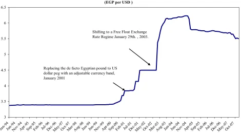
In January 2001; Egypt replaced the de facto Egyptian pound to US dollar peg with an adjustable currency band, where the Egyptian pound gradually lost about 48 percent of its value against the US dollar over the period 2001-2003. (ERF and IM 2004)
On January 29, 2003, the adjustable peg was swapped with a floating exchange rate regime (See figure 4). Under the free float, banks were permitted to determine the buy and sell prices of exchange rates. The CBE was barred from intervention in setting the foreign exchange rate, except to correct for major imbalances and sharp swings (El-Asrag 2003).
Source: CBE data.
Despite the liberalization of the pound in 2003, the CBE has continued to maintain exchange rate stability as one of its key objectives during the following years, 2004 till 2007. Suspecting that further going; the CBE might still choose to keep a tight grip on the foreign exchange market.
In theory, efficient monetary policymaking, however, tolerates intervention in the foreign exchange market only by means of policy measures. So far, the CBE has a good record on that account. For instance, the fears of dollarization that followed the liberalization of the pound, prompted the CBE to tighten monetary policy through an increase in the rate of interest (CBE 2004/2005).
Starting from 2006 and going forward; the main objective of the CBE has been to keep inflation low and stable. That objective was cast within the context of a general program to move eventually toward anchoring monetary policy by inflation-targeting once the fundamental machinery needed for its implementation is installed (CBE 2005).
[image:30.612.75.545.92.351.2]Meanwhile, in the transition period, the CBE intends to meet its inflation stabilization objective through the management of the short-term interest rates and the control of other factors that affect the inflation rate including shocks to credit and to money supply (CBE 2005).
Figure 4: Nominal Exchange Rate (EGP per USD )
3 3.5 4 4.5 5 5.5 6 6.5 Jan-9 4 Jun-9 4 Nov -94 Apr-9 5 Se p-95 Feb-9 6 Jul-9 6 Dec-9 6 May -97 Oct-9 7 Ma r-98 Aug-9 8 Jan-9 9 Jun-9 9 No v-99 Apr-0 0 Sep-0 0 Feb-0 1 Jul-0 1 Dec-0 1 May -02 Oct -02 Ma r-03 Aug-0 3 Jan-0 4 Jun-0 4 Nov -04 Apr -05 Se p-05 Feb-0 6 Jul-0 6 Dec-0 6 May -07 Oct -07 Shifting to a Free Float Exchange
Rate Regime January 29th. , 2003.
In view of the recent changes in policymaking initiated by the CBE, we anticipate that the upcoming period shall witness important actions to conduct monetary policy on objective and methodical bases.
Believing that good measurement of monetary policy and of the stance within the last 15 years or so should provide a suitable inferential point of departure en route toward the support of those actions.
B- Constructing the model
1- The data
• The output gap: for the actual output; the industrial production (from the CAPMAS) is
used (on a quarterly basis34) as a proxy for the actual GDP, as it represents the largest
compound of the GDP (around 18 percent during 2007)35. For the potential output, we
applied the HP filter technique to derive the potential output from the selected actual
output series36.
• The central bank policy rate (nominal interest rate): From the mid-1980s to 2007, the
CBE used different rates of interest as policy instruments. For example; the discount rate, the 3-month deposit rate, the Treasury Bills rate and the interbank overnight rate. To maintain a sufficient number of degrees of freedom, it would not be practically feasible to take account of all these interest rates concurrently in a VAR model. We picked the 3-month deposit rate (from the Central Bank of Egypt) to represent the
interest rate component of the CBE operating procedure37.
• The inflation rate: we selected the year-on-year monthly inflation rate based on the
Consumer Price Index (CPI) (from the CAPMAS), rather than any other inflation index as the Whole Price Index (WPI) for two reasons. First: most of the related studies use the CPI while estimating the interest rate rule. Second: the CAPMAS stopped the WPI series in November 2007; on the other hand, it started to issue a new series regarding the Producer Price Index (PPI) instead.
• The long-run equilibrium real interest rate: this constant value is calculated as
follows: first: derived the long-run path of the 3-month domestic deposit rate using the
HP filter technique, second: we calculated the simple average of the derived long-run
path to get the natural rate of return.
• The exchange rate: for this variable, we followed the other related studies to use the
real effective exchange rate (REER) of the Egyptian pound38 (an increase means an
appreciation), while estimating the interest rate rule in Egypt.
34
The quarterly series is converted to a monthly one using the E-views frequency conversion technique (Quadratic-match average).
35
Source: Central Bank of Egypt web-site
36
Although the limitation of the HP filter technique, regarding the constant parameter (λ) which controls the smoothness of the trend component (λ = 14400 for monthly data), but it gave better results than other techniques as Nadaraya-Watson detrending technique.
37 It represents the most consistent series, while the Treasury Bills and the interbank overnight rate policy instruments were introduced in different periods; the selected time horizon for analyzing the movement in those instruments differs accordingly.
38
Table 1 in appendix A, show the data spread sheet. Also, Figures 1 to 3 in the mean appendix, represent the movements in both CPI inflation rate and 3-month deposits rate, industrial production and its potential detrended series, and nominal exchange rate and REER, respectively.
Table 2: Data description
Variable Description
I 3-month Deposit rate (%)
CPI Consumer Price Index Inflation rate (y-on-y) (%) IP Industrial Production (in million EGP)
YPOTEN Potential Industrial Production (Output) using hp-trending LREER Log Real Effective Exchange rate using CPI (%)
DV_REER Dummy Variable (DV_REER= 1 starting from 2003:01, and zero otherwise) YGAP The output gap ( IP – YPOTEN )
2- Methodology: the models
i- The first model: The central banks` reaction function
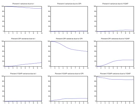
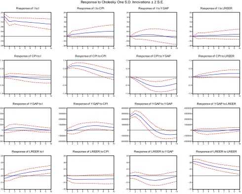
In this context, we estimated the central bank reaction function in the case of both closed and open economy, using the vector autoregression (VAR) technique to show the short-run relation between the variables. This relation can be shown by the impulse response function derived from the VAR, to exam the effect of the inflation, output gap and the exchange rate shocks on the interest rate. In addition, the variance decomposition is derived to show how much variation in the nominal interest rate as a monetary policy instrument is attributed to the different shocks.
Equations (1)-(4) illustrated in part three and the relevant parametric restrictions were employed to estimate the parameters of an un-structural VAR for each of both closed and open economy models described above in part three. The VAR estimates are obtained using monthly data for Egypt during the period 1997-2007.
The paper follows the academic literature that has tried to identify monetary policy shocks. Thus, in common with previous research, the paper use variables those are in
levels.39
39
The central banks` reaction functions in a closed economy
Table 2 in appendix C; reports the un-structural VAR parameter estimates and their standard errors obtained from the closed economy model. The un-structural VAR specification was fit with 8 lags in levels of the 3-month deposits rate, CPI and the output
gap40.
The closed economy VAR Model representation:
================================================
I = C(1,1)*I(-1) + C(1,2)*I(-2) + C(1,3)*I(-3) + C(1,4)*I(-4) + C(1,5)*I(-5) + C(1,6)*I(-6) + C(1,7)*I(-7) + C(1,8)*I(-8) + C(1,9)*CPI(-1) + C(1,10)*CPI(-2) + C(1,11)*CPI(-3) + C(1,12)*CPI(-4) + C(1,13)*CPI(-5) + C(1,14)*CPI(-6) + C(1,15)*CPI(-7) + C(1,16)*CPI(-8) + C(1,17)*YGAP(-1) + C(1,18)*YGAP(-2) + C(1,19)*YGAP(-3) + C(1,20)*YGAP(-4) + C(1,21)*YGAP(-5) + C(1,22)*YGAP(-6) + C(1,23)*YGAP(-7) + C(1,24)*YGAP(-8) + C(1,25)
CPI = C(2,1)*I(-1) + C(2,2)*I(-2) + C(2,3)*I(-3) + C(2,4)*I(-4) + C(2,5)*I(-5) + C(2,6)*I(-6) + C(2,7)*I(-7) + C(2,8)*I(-8) + C(2,9)*CPI(-1) + C(2,10)*CPI(-2) + C(2,11)*CPI(-3) + C(2,12)*CPI(-4) + C(2,13)*CPI(-5) + C(2,14)*CPI(-6) + C(2,15)*CPI(-7) + C(2,16)*CPI(-8) + C(2,17)*YGAP(-1) + C(2,18)*YGAP(-2) + C(2,19)*YGAP(-3) + C(2,20)*YGAP(-4) + C(2,21)*YGAP(-5) + C(2,22)*YGAP(-6) + C(2,23)*YGAP(-7) + C(2,24)*YGAP(-8) + C(2,25)
YGAP = C(3,1)*I(-1) + C(3,2)*I(-2) + C(3,3)*I(-3) + C(3,4)*I(-4) + C(3,5)*I(-5) + C(3,6)*I(-6) + C(3,7)*I(-7) + C(3,8)*I(-8) + C(3,9)*CPI(-1) + C(3,10)*CPI(-2) + C(3,11)*CPI(-3) + C(3,12)*CPI(-4) + C(3,13)*CPI(-5) + C(3,14)*CPI(-6) + C(3,15)*CPI(-7) + C(3,16)*CPI(-8) + C(3,17)*YGAP(-1) + C(3,18)*YGAP(-2) + C(3,19)*YGAP(-3) + C(3,20)*YGAP(-4) + C(3,21)*YGAP(-5) + C(3,22)*YGAP(-6) + C(3,23)*YGAP(-7) + C(3,24)*YGAP(-8) + C(3,25)
40
- .10 - .05 .00 .05 .10 .15 .20 .25
1 2 3 4 5 6 7 8 9 10
Response of I to I
-.10 -.05 .00 .05 .10 .15 .20 .25
1 2 3 4 5 6 7 8 9 10
Response of I to CPI
- .10 - .05 .00 .05 .10 .15 .20 .25
1 2 3 4 5 6 7 8 9 10
Response of I to YGAP
- 0.8 - 0.4 0.0 0.4 0.8 1.2
1 2 3 4 5 6 7 8 9 10
Response of CPI to I
-0.8 -0.4 0.0 0.4 0.8 1.2
1 2 3 4 5 6 7 8 9 10
Response of CPI to CPI
- 0.8 - 0.4 0.0 0.4 0.8 1.2
1 2 3 4 5 6 7 8 9 10
Response of CPI to YGAP
-2000000 -1000000 0 1000000 2000000 3000000 4000000
1 2 3 4 5 6 7 8 9 10
Response of Y GAP to I
-2000000 -1000000 0 1000000 2000000 3000000 4000000
1 2 3 4 5 6 7 8 9 10
Response of YGAP to CPI
-2000000 -1000000 0 1000000 2000000 3000000 4000000
1 2 3 4 5 6 7 8 9 10
Response of YGAP to YGAP
[image:35.612.114.522.118.442.2]Respons e to Choles ky One S.D. Innovations ± 2 S.E.
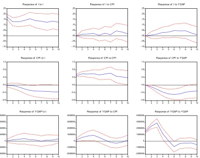
Figure 5: Impulse response functions
Figure 5 above, shows the impulse response functions of the 3-month deposits rate, CPI inflation rate, and output gap. Compromises two important findings:
1- The response of CPI to both the interest rate and output gap shocks will have a
continuous negative impact. Alternatively, a weak41 positive continuous impact of
interest rate to a CPI shock is determined.
2- No long-run impact of interest rate on the output gap, as the model implies very weak
effects for the interest rate shock on output gap during the sample period, which will die after six months.
On the other hand, the model shows a significant response of the output-gap to a price shock, which will also; vanish after six periods (no long-run impact).
41