High Dimensional Dataset Compression Using Principal Components

(1)

High Dimensional Dataset Compression Using

Principal Components

Michael B. Richman1, Andrew E. Mercer2, Lance M. Leslie1, Charles A. Doswell III3, Chad M. Shafer4

1_{School of Meteorology, University of Oklahoma, Norman, USA} 2_{Department of Geosciences, Mississippi State University, Starkville, USA} 3_{Cooperative Institute for Mesoscale Meteorological Studies, Norman, USA} 4_{Department of Earth Sciences, University of South Alabama, Mobile, USA}

Email: [email protected]

Received May 11, 2013; revised June 11, 2013; accepted June 18,2013

Li-cense, which permits unrestricted use, distribution, and reproduction in any medium, provided the original work is properly cited.

ABSTRACT

Until recently, computational power was insufficient to diagonalize atmospheric datasets of order 108_{- 10}9_elements.

Eigenanalysis of tens of thousands of variables now can achieve massive data compression for spatial fields with strong correlation properties. Application of eigenanalysis to 26,394 variable dimensions, for three severe weather datasets (tornado, hail and wind) retains 9 - 11 principal components explaining 42% - 52% of the variability. Rotated principal components (RPCs) detect localized coherent data variance structures for each outbreak type and are related to standardized anomalies of the meteorological fields. Our analyses of the RPC loadings and scores show that these graphical displays can efficiently reduce and interpret large datasets. Data is analyzed 24 hours prior to severe weather as a forecasting aid. RPC loadings of sea-level pressure fields show different morphology loadings for each outbreak type. Analysis of low level moisture and temperature RPCs suggests moisture fields for hail and wind which are more related than for tornado outbreaks. Consequently, these patterns can identify precursors of severe weather and discriminate between tornadic and non-tornadic outbreaks.

Keywords: Data Compression; Eigenanalysis; Computational Complexity; Severe Weather; Rotated Principal

Components

1. Introduction

Principal Component Analysis (PCA) has been used ex- tensively in the atmospheric sciences for over 60 years [1-4]. The value of PCA in atmospheric sciences applica- tions stems from the compact description of space-time- variable datasets into two graphical displays that convey the dominant patterns of space variation and their associated time behavior. One challenge of using PCA is its high computational time complexity. Numerical models often measure variables on grids of L latitudes by M lon- gitudes by N vertical levels, with LxMxN gridpoints, with model output at T times. This leads to a data matrix of either T x (LxMxN) or (LxMxN) x T for each model va-

riable, P.Since LxMxN is often of order 108_{, an eigende-}

composition of the model output can be a daunting task,

since PCA requires O((LxMxNxP)3_{) computations. With}

ten variables typically being analyzed simultaneously,

this can lead to matrix diagonalizations of the order 109_.

The models are expected to exceed 1010_{in the near future.}

(2)

mension of the data matrix, leading to a limited number of eigenmodes. In the present application, we seek to analyze the (LxMxNxP) dimension to determine group- ings of those variables that have similar time evolutions for severe weather outbreak types [9-12]. In so doing, we obtain modes of variability in the three-dimensional atmosphere that corresponds to 24 hours prior to the onset of severe weather, useful to forecasters. Forecasting severe weather a day before it occurs is controlled largely by atmospheric spatial scales exceeding approximately 2000 km in distance (referred to by meteorologists as synoptic scale or larger). Data over such an area represent a nearly instantaneous snap-shot of the state of the atmosphere and the features at this scale tend to persist long enough to enhance predictability. If the validity of eigen- structures at these space scales is established, they can be investigated as precursors of the outbreaks. Knowledge of such patterns can assist in forecasting the location of the severe weather a day or more in advance of the outbreak, thereby providing the potential to reduce casual- ties.

2. Data and Methods

2.1. Defining Outbreaks

Prior to formulating composites of the different outbreak types, a formal definition of each outbreak type was required. Following the ranking methods outlined in [13], the N15 ranking index of outbreaks was used to assess significant tornado outbreaks. In particular, outbreaks with an N15 ranking index of 2 or higher that included 6 or more Storm Prediction Center (SPC) tornado reports were considered as “major” tornado outbreaks. However, since the N15 ranking index was developed based on criteria relevant for tornado outbreak severity (e.g. the number of tornadoes that cause death, the number of significant tornadoes, etc.), using this scheme for ranking hail and wind-dominated outbreaks was not appropriate. Since no formal ranking approach exists for these outbreak types, a simple relationship comparing the number of wind reports and hail reports was utilized to define each group. In particular, outbreaks whose number of wind reports exceeded three times the number of hail reports that had an N15 ranking of less than 2 (thereby excluding them from the tornado group) were considered “major” wind outbreaks, while outbreaks with three times the number of hail reports as wind reports with an N15 index < 2 were considered “major” hail outbreaks. Through the use of these criteria, sets of 79 tornado outbreaks, 131 wind outbreaks, and 245 hail outbreaks were defined for the time dimension.

2.2. Data and Analysis Procedure

High dimensional studies require some modification of

the typical eigenanalysis methodology. Prior to the data reduction, rather than examining scalar values, graphical methods are employed where possible. The steps in the analysis are: (1) decision on the type of analysis dictated by research question, (2) sampling available data, (3) qua- lity control and missing data, (4) remapping the data to an unbiased grid, (5) scaling the data, if necessary, (6) formation of a similarity matrix, (7) diagonalization of similarity matrix, (8) selecting a range of the number of eigenvectors, (9) formation of unrotated principal component loadings, (10) rotation of different numbers (from step 7) of unrotated PC loadings to select the most appropriate number of rotated PC loading vectors, (11) ex- traction of rotated PC scores and (12) physical interpretation of the results.

Step 1. Our research goal is to identify recurring patterns of atmospheric variables associated with tornado, hail and wind severe weather outbreaks. This is a space- time analysis of the three-dimensional atmosphere and we form a multilevel set of grids in the data matrices, with the spatial gridpoint values of the variables as columns and the outbreak cases as rows. The NCEP/NCAR reanalysis project (NNRP) [14] provides three-dimensional global reanalyses of numerous meteorological variables, relevant to severe weather formation. The dataset

is defined by a horizontal (LxM) 2.5˚ latitude-longitude

grid spacing with 17 vertical levels (N) and over the entire globe at 6 hour time intervals from 1948 to present. For this study, three-dimensional fields of geopotential height, specific humidity, zonal and meridional wind components, were obtained for a study domain centered on

North America (Figure 1) for each outbreak type. Four

of the variables: geopotential height, temperature, zonal and meridional wind were measured at all 17 levels (4 × 17 = 68 of the 83 variables). The specific humidity data are not provided at pressure levels less than 300 hPa; therefore, the eight levels closest to the surface were selected. Additionally, there were seven surface variables (mean sea-level pressure, surface pressure, temperature, zonal and meridional wind components for a total of 68 + 8 + 7 = 83 variables for each gridpoint. Variables were obtained 24 hours prior to the valid time of the outbreak

to construct each outbreak type matrix (i.e., tornado, hail,

wind). Hence, these matrices provide information on the pre-outbreak atmosphere, a time frame that is particularly useful to severe weather forecasters or pattern recognition algorithms looking for outbreak precursors.

Step 2. Data from the beginning of the NNRP record until the last date available were used in this study. There- fore, our sample is the finite population of all reanalysis data.

(3)

Step 4. The NNRP are provided on a latitude-longitude

grid (Figure 1(a)). The goal of the analyses is to provide

modes of variability of the spatial coherence of the data. Owing to the poleward convergence of the longitude lin- es in the NNRP data, there is an artificial inflation of as-

sociation among nearby gridpoints (i.e., their covariances)

that is a function of latitude. As eigenanalysis is a decomposition of the variance structure of the data, it is necessary to remove this source of bias by interpolating

to a Fibonacci grid [15] (Figure 1(b)), by providing

equally spaced gridpoints over the entire domain (318 Fi- bonacci gridpoints). Three final datasets resulted from these analyses, consisting of all gridpoints (ordered longitude-latitude-level-variable) along the columns of each matrix (26,394 columns) and the events on the rows (numbers match number of outbreaks of each type). This defines an S-mode analysis [16].

Step 5. Because the variables have vastly different

units and values (e.g. specific humidity ~ 1 × 10−3_kg/kg

versus geopotential height at 500 hPa ~ 5400 m), the data were pre-standardized through z-score calculations ateach vertical level and for each variable prior to place

(a)

(b)

Figure 1. The study domain on the original NNRP grid (a) and on the Fibonacci grid (b).

ment in the data matrices that were to be eigenanalyzed. Since the data were standardized to a zero mean and unit standard deviation at each vertical level to account for the varied units and large variation in the values as a function of pressure level, values in the data matrices are

standardized anomalies (Z).

Step 6. As values in the data matrices are standardized

anomalies (Z) from the mean (step 5), similarity is mea-

sured by forming correlation matrices (R) of order 26,394.

Three correlation matrices are formed for tornado, hail and wind outbreaks.

Step 7. Each correlation matrix was decomposed into a

square matrix of eigenvectors (V) and associated diago-

nal matrix of eigenvalues (D), given by the decomposi-

tion

 T

R VDV (1)

Step 8. The rank of the eigenvector matrix is equal to

the smaller of the number of gridpoints (n) or number of

observations (m) minus 1. Because there were m = 79

observations for tornado outbreaks, only 78 eigenvalues were nonzero and 78 eigenvectors were extracted. Simi-larly, 244 (130) non-zero eigenvalues existed for the hail (wind) outbreaks. The goal of this stage of the analysis is to create a set of basis vectors that compress the original

variability in R into a new reference frame. It is possible

to plot the n elements of each eigenvector (V) on spatial

maps; however, the patterns in V do not result in any

localization of the spatial variance, nor do they represent

well the variability in R [16].

For high dimensional problems, interpretation requires that the analyst must explain the relationships among many thousands of variables for each eigenvector retained. The eigenvectors are ordered indexed by decreasing eigenvalue. Many of the 78 eigenvectors depict small- scale (sub-synoptic scale) signals with variance properties indistinguishable from noise, having very small eigenvalues. We truncate the number of principal components to represent only that variance associated with synoptic scales or larger that correspond to spatial patterns present in the 26,394 × 26,394 correlation matrix, using a two step process. First, the magnitudes of the eigenvalues are examined and those with relatively large eigenvalues

are retained to yield a subset of l principal component

loading vectors. The value l is selected by implementing

the scree [17] and standard error tests [4] to provide a vi- sual estimate of the approximate number of non-degen-

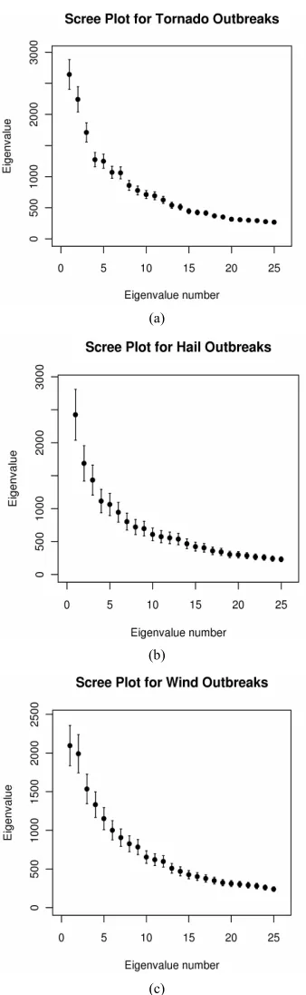
erate eigenvectors to retain. Figure 2 shows the results of

[image:3.595.59.285.368.703.2]

(4)

(a)

(b)

[image:4.595.87.256.79.627.2]

(c)

Figure 2. Scree test plots of eigenvalue number against ei- genvalue magnitudes for tornadoes (a), hail (b) and wind (c) outbreaks. The error bars represent the 95% CI for each eigenvalue.

Owing to the aforementioned degeneracy, a number of

roots retained, l, is selected liberally, intentionally repre-

senting more than the ideal number of roots, k, associated

with the signals representing spatial scales of at least the

synoptic-scale.

Step 9. As the magnitude of the eigenvector elements

varies as a function of the number of variables (n), the

eigenvectors (V) were scaled by the square root of the

corresponding eigenvalue, VD1/2 to create principal com-

ponent loadings (A). Doing so converts the eigenvectors

to units of the similarity matrix (i.e., correlations) with a

known range and permits the data to be expressed as

 T

Z FA (2)

where the vectors in F represent the new set of basis

functions, known as principal component scores and A is

the matrix of weights that relates the original standard-

ized data (Z) to F. The vectors in A contain elements that

are correlation coefficients between Z and F.

Step 10. To assess the coherency gained through loca-

lization of the signal, the l vectors identified in A are

post-processed by linearly transforming them to a new

set of vectors, B, known as rotated principal component

(RPC) loadings. The rotation of PC loadings simplifies or localizes the variables by finding the orientation of the PCs that results in many of the variables having small projections or loading values and other variables having large projections. Such simplified loadings correspond better with the correlation structure of the data [16], en- hancing physical interpretation. The rotation process can be summarized by the equation



B AT (3)

where T is an invertible kxk orthonormal transformation

matrix that represents a rotation of the reference frame into a position that results in the greatest simplification in

the vectors of B. Then from (3)

 

T T T

BB ATT A AAT (4)

and from (1) and (2), B represents the similarity matrix

or data set as does A. Moreover, an infinite number of

transformation matrices will satisfy (4); therefore, some additional constraint is required. For high dimensional

problems, it is desirable to find T that simplifies each

vector, B, as much as the data permit. Doing so allows

for a smaller subset of variables (as opposed to tens of

thousands) to be interpreted for each column of B. For

our problem, the column vectors in B are plotted on a

spatial map, and the simplification corresponds to detect- ing localizations of coherent signal in standardized anomaly patterns that recur often in the correlation structure of the variables. The rotation algorithm used in this analysis is Varimax [16]. Varimax is termed an “orthogonal”

rotation, indicating the transformation matrix (T) in (3) is

orthogonal as TTT = I. The Varimax simplification algo-

rithm maximizes the variance, of the PC loadings,

and is given by

2 v

2

i b

 

2

 

2

2 2 2 2

2

1 1 1 1

1 1

k k n n

j ij

j j i i

v v b b

n n

    ij

 

  _  _

 

(5)

This algorithm proceeds with a planar rotation of all possible pairs of PC loading vectors and maximizing

in (5). Once the final is achieved, the solution is

simplified in the sense that each column of B corre-

sponds to the solution that maximizes simultaneously the

number of near-zero loadings and large load-

ings , while minimizing the number of moderate

magnitude loadings. Values of i near-zero explain lit-

tle variance, , for a given PC loading vector j in B and

those variables with near-zero loadings, for a given PC loading vector, do not need to be interpreted. This solu- tions that result from a Varimax rotation are characterized by groups of variables having high magnitude loadings on one PC and other groups of variables with high magnitude loadings on a different PC loading vector.

Since _j_₁ for the correlation-based analysis,

most of the variable’s variance is accounted for in a Va- rimax solution, when the loadings are large.

2 v 2

v



bij 0

b





bij1

b k i b



2 i 1

Given the high dimensionality of the problem (the

26,394 row entries in B) the larger the number of near-

zero and large i , the more binary (simpler) solution

leads to easier the interpretation loadings in a Varimax solution. The simplicity of the solution is seen by inspec-tion of the density funcinspec-tions for the PC loadings before

and after rotation. Figure 3 shows the empirical probabi-

lity density functions (PDFs) concentration of near-zero loadings for the rotated solution in comparison to the unrotated solution for the first PC for tornado outbreaks.

The improved simplicity, seen in Figure 3, is document-

ed in Table 1 for all PCs and outbreak types by examin-

ing the kurtosis of the loadings before and after rotation. Most unrotated PC loading vectors had platy-kurtotic or mesokurtotic distributions; whereas, after rotation, the di-

stributions become leptokurtotic (Table 1), reflecting the

more simplified (peaked) distributions. When the columns

of Varimax loadings are mapped to the grid (Figure 1(b)),

b s

PC Loading Magnitude Tornado PC Loading Density

-1.0 0.0 0.5 2.0 Pr o b a b ility ( P e rce n t)

-0.5 0.0 0.5 1.0

red = unrotated blue = rotated

1.

0

[image:5.595.309.538.111.338.2]

1.5

Figure 3. Empirical PDFs for PC loading vector 1 unrotated (red) and Varimax rotated (blue).

Table 1. Kurtosis statistics for PC loading vectors of tor- nado, hail and wind outbreaks.

Unrotated Kurtosis Rotated Kurtosis PC

Tornado Hail Wind Tornado Hail Wind

1 −0.51 −0.10 −0.05 0.66 0.72 1.15

2 −0.40 −0.21 −0.31 0.75 1.43 1.37

3 −0.52 −0.12 −0.56 0.32 2.14 1.41

4 −0.45 −0.14 −0.18 0.84 1.15 1.14

5 0.12 −0.21 −0.20 2.32 0.83 1.37

6 0.96 0.26 −0.16 1.65 0.55 0.13

7 −0.09 −0.24 −0.27 0.52 1.31 1.72

8 −0.44 0.03 0.25 0.45 2.18 1..01

9 −0.30 −0.05 −0.14 1.02 1.09 1.47

10 0.14 -- −0.18 0.31 -- 0.54

11 -- -- −0.21 -- -- 3.13

the large loadings are grouped in isolated clusters with areas on near-zero loadings between the clusters, accor- ding to the correlation structure of the data. This process of rotation and mapping makes analyzing high dimensional problems tractable and is amenable to physical interpretation.

The spatial properties of each vector in B depend on

the number of rotated PC vectors retained (l). Therefore,

it is critical to select the optimal number of vectors, k,

that correspond to data signal and reject small-scale noise

from eigenvalues k + 1 to the dimension associated with

the order on R.

To accomplish that goal, the matrix A is transformed

to B for a variable number of retained RPC vectors (i.e.,

2 to l). Each solution, based on a different number of

RPCs, yields a different set of patterns when the elements

of B are mapped back to the Fibonacci grid. We require a

set k < l that captures as much coherent large scale signal

as possible that matches the patterns embedded within R.

The one set of k PC loadings that relates best to the cor-

relation matrix generating them is determined and the

number of PCs retained is set to k.

The process, outlined in [18], and refined in [16], se-

lects each vector in B and identifies the location or grid-

point associated with the largest absolute RPC loading. Next, the RPC loading vector is matched to the vector in

R corresponding to the gridpoint identified with the ma-

ximum absolute loading. This method incorporates the

logic that the solution associated with k PCs must have

spatial structures that match optimally to those spatial

structures in R. An additional advantage to post-process-

[image:5.595.61.287.531.705.2]

(6)

position to eigenvector degeneracy [18]. The two vectors are matched, through the congruence coefficient [16], a scalar quantity that is the uncentered correlation coefficient (or the cosine of the geometric angle between the two vectors). The congruence coefficient measures both phase and magnitude match. The values of congruence

range from −1 to +1, with +1 being a perfect match. The

application of the congruence coefficient in this manner

provides an objective procedure to select k objectively.

For the tornadic outbreak set, the Varimax solution with

the optimum match occurred as k = 10 (average congru-

ence was 0.90) associated with 51.5% of the explained variance, for the hail outbreak set the optimum match

was at k = 9 (average congruence was 0.91) with 41.2%

of the explained variance and for the wind data set, k =

11 (average congruence was 0.92) with 48.9% of the explained variance. Thus, among these datasets, the data compression was impressive (12.8%, 3.6% and 8.5% of the basis vectors associated with non-zero eigenvalues of tornadoes, hail and wind outbreaks accounted for 51.5%, 41.2% and 48.9% of the total variance, respectively).

Step 11. Once the spatial patterns have been identified, the projections of the standardized data on the loadings are calculated to obtain the amount of each RPC pattern associated with each outbreak (e.g., how much of RPC 1 exists in the outbreak 1 for tornadoes?). To accomplish

this, the RPC scores (F) are calculated as

 



 T 1

F ZB B B (6)

The PC scores are in units of standard deviations from the mean.

Step 12. A physical interpretation of the standardized anomaly fields associated with each mode involves mul- tiplying the PC score is by the PC loading [7]. For exam- ple, a negative anomaly in a RPC loading map of geopotential multiplied by a negative PC score gives the interpretation of a positive height anomaly. Interpretation of the graphical and mapped RPC loadings and time series of the RPC scores will now be presented.

3. Interpretation of RPCA of Severe

Weather Outbreak Types

3.1. Scatterplot Analysis of RPC Loadings

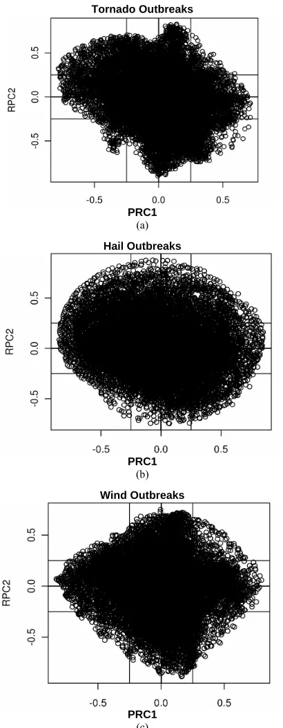
Normally, for datasets with a small number of variables, the RPC loadings are inspected in a table and similarities noted. However, in the present analysis, there are 26,394 elements for each loading vector, making a tabular in-spection of each element intractable. To assess the co-herence of the loadings for such a large number of ele-ments requires a graphical technique that plots the RPC loadings for each vector retained as a biplot or scatterplot. The goal is to investigate whether the variables cluster into coherent groups that can be interpreted when

mapped back to the Fibonacci grid. Because PC (or RPC) loading values of < |0.25| are considered essentially sampling deviations from zero [19], those variables exist in a hyperplane of width ± 0.25. Interpretation of the scatterplots of the pairs of PC loadings (the first two for each

outbreak type are shown in Figure 4) indicates that the

Tornado Outbreaks

PRC1 (a)

Hail Outbreaks

PRC1 (b)

Wind Outbreaks

[image:6.595.320.525.169.695.2]

PRC1 (c)

(7)

majority of variables exist close to the origin of the graph, within the hyperplane.

For the tornado outbreaks (Figure 4), there is a clear

orientation of variables along the RPC axes in the x- and y-axis directions, suggesting well-defined modes of variation as the axes represent the RPCs. In contrast, the hail outbreaks exhibit more of a “bulls-eye” pattern with the highest concentration in the hyperplane and less dis-

tinct clustering along the RPC axes (Figure 4). This con-

figuration of variables is indicative of the lower variance

explained in hail events. The wind outbreaks plot (Fig-

ure 4) has a configuration of clustering along the RPC

axes, consistent with the higher amount of variance ex-

plained with fewer PCs retained. Overall, Figure 4 de-

monstrates that modes of variation have clusters of variables that can be investigated further in spatial analyses of the RPC loadings plotted on the Fibonacci grids and the associated time series graphics.

3.2. Interpretation of the RPC Loading Maps for Each Outbreak Type

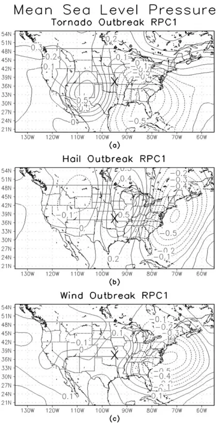
[image:7.595.311.536.82.518.2]

The outbreak RPC loadings can be interpreted when plotted to the Fibonacci grids and then isoplethed to produce fields of the variables. As there are 83 variables per outbreak type, three outbreak types with 9, 10 and 11 RPCs, that is 83 × 30 maps of PC loadings. Since the atmosphere is sampled for many variables in 3-dimensions, it is possible to examine many additional vertical slice maps. We will present just a small fraction of the results to il- lustrate the differences in the physical meteorological variables as a function of outbreak type. The mean sea- level pressure for the three outbreak types is shown in

Figure 5. Convective storms are often linked to cyclones

that are associated with relatively low pressure. Such cyclones induce low-level convergence and the associated vertical motion. It is important to note that these maps are generated for data that were collected 24 hours prior to the onset of the outbreak. Hence these are precursor fields. Additionally, the grid the data are placed on was moved to be centered on the outbreak centroid. Therefore,

the “X” in Figure 5 in southeastern Kansas, meant to

show the center of the outbreak is not referenced to the specific geographical location; rather, the map is provided to convey an idea of the spatial scale and configurations of the RPC loading anomalies relative to the center of the outbreak.

Tornado outbreaks (Figure 5(a)) are characterized by

negative RPC loadings to the east of the outbreak and positive loadings to the west of the outbreak. Since the sign of the loadings is arbitrary, there is ambiguity in the

sign of the anomalies in Figure 5 and the RPC scores

must be examined for each outbreak to assign a sign to that case. For tornadic outbreak cases with positive large

Figure 5. RPC loadings of mean sea level pressure for tor- nado (a), hail (b) and wind outbreaks (c).

magnitude RPC scores, the physical interpretation would be anomalously high pressure to the east and anomalously low pressure to the west. Conversely, for cases with large negative RPC scores, the interpretation would be anomalously high pressure to the east and anomalously low pressure to the west. Twenty-four hours prior to the tornado outbreaks, the center of the outbreak is on a zero line between the two anomalies. In contrast, for hail out-

breaks (Figure 5(b)), there is a tripole pattern of sea-le-

(8)

for a large magnitude positive or negative sign and inde- xing the RPC loading sign accordingly. Unlike the previous two outbreak maps, the wind outbreaks have a much weaker gradient of RPC loadings in the east-west

direction (Figure 5(c)) with the center of the outbreak

located in an area of weakly positive PC loadings. Recall, in the discussion of hyperplanes, any PC loading with an absolute magnitude of less than 0.25 is considered essentially zero. Therefore, the loadings to the west of the center of the outbreak correspond to near-zero anomalous

pressure. Examination of the three plots in Figure 5 sug-

gests that the sea-level pressure patterns, associated with the three outbreak types 24 hours prior to the onset of the outbreak, have different in spatial structures.

Another ingredient in severe weather outbreaks is the availability of moisture for convection. The measure of moisture used in this study is specific humidity at the 850

hPa level and is shown for the three outbreak types in Fi-

gure 6. As was the case for the sea-level pressure, these

moisture data were collected 24 hours prior to the onset of the outbreak. Unlike the pressure fields, the moisture fields have a more common pattern with smaller differ-ences in the patterns for outbreak types. For tornado

out-breaks (Figure 6(a)) the RPC pattern has a negative ano-

maly to the southwest of the outbreak centroid, indicative of drier than average air in that location. Since the sign of the loadings is arbitrary, the sign of the anomalies requires inspecting the RPC score for any given outbreak. If that score has a large positive value, the pattern on the map is likely to be found. Alternately, for cases with large negative RPC scores, the interpretation would be anomalously moist region to the southwest of the outbreak. The leading RPC specific humidity pattern associated

with hail outbreaks (Figure 6(b)) indicates a spatially ex-

tensive anomaly centered to the east northeast of the outbreak center with a strong PC loading gradient over the outbreak area. The wind outbreak RPC of specific humi-

dity (Figure 6(c)) has a spatially extensive anomaly of

loadings centered to the east of the outbreak centroid. The difference between the hail and wind outbreak patterns is the lack of a strong gradient in the latter. The third field being investigated is air temperature at 850

hPa (Figure 7). Since 850 hPa is situated relatively low

in the troposphere, it gives an indication of low-level thermal properties. The change in the pattern over time is considered important for assessing the instability of the atmosphere. As for the previous two fields, these temperature data were collected 24 hours prior to the onset of the outbreak. The leading RPC loadings for the tempera-

ture field taken from the tornado outbreaks (Figure 7(a))

has a negative anomaly to the south of the outbreak centroid, indicative of cooler than average air in that location. Additionally, about 1500 km to the west of the outbreak center, there is a region of positive RPC loadings, indi-

Figure 6. RPC loadings of 850 hPa specific humidity for tor- nado (a), hail (b) and wind outbreaks (c).

cative of anomalously warm air. As before, since the sign of the loadings is arbitrary, the sign of the anomalies requires inspecting the RPC score for any given outbreak. If that score has a large positive value, the pattern on the map is likely to be found. Alternately, for cases with large negative RPC scores, the interpretation would be anomalously warm region to the south of the outbreak and a cool anomaly to the west. The leading RPC 850 hPa temperature pattern associated with hail outbreaks (Figure 7(b)) and wind outbreaks (Figure 7(c)) have si-

(9)

[image:9.595.60.285.87.546.2]

Figure 7. RPC loadings of 850 hPa temperatures for tor- nado (a), hail (b) and wind outbreaks (c).

3.3. Interpretation of RPC Score Time Series for Each Outbreak Type

Because this is a multi-field PCA, the RPC scores average all the fields in (6) with equal weight to generate standardized scores; fields with fewer levels, such as the surface variables will be represented less than those fields with 17 levels. Typically, examining the extreme

positive (scores ≥ 1) and negative values (scores ≤ −1)

and then identifying the outbreak cases that correspond to the extreme values facilitate interpretation of the RPC

scores. The tornado outbreak RPC 1 score plot (Figure 8)

indicates there are multiple outbreaks that have patterns

similar to the RPC 1 loadings. The first RPC score clas- sifies 12 (of the 79) cases (15.2%) as having spatial configurations of the standardized anomaly patterns of the

variables similar to the maps shows in Figures 5-7. Only

3 of the outbreaks occurred with the spatial patterns of opposite signs to those shown in the aforementioned figures.

As suggested by the lower degree of clustering for the

scatterplots of PC loadings for hail (Figure 4(b)), the

hail outbreak RPC 1 score plot (Figure 9) reveals a more

variable pattern compared to the tornado outbreaks. The hail outbreak scores have 41 cases (16.7%) with scores greater than or equal to 1 and 16 cases (6.5%) with

scores less than or equal to −1. There is evidence in the

meteorological literature that hail events can occur with varied atmospheric patterns [20]. The events with extreme scores can have their standardized anomalies com-

pared to the spatial patterns in Figures 5-7.

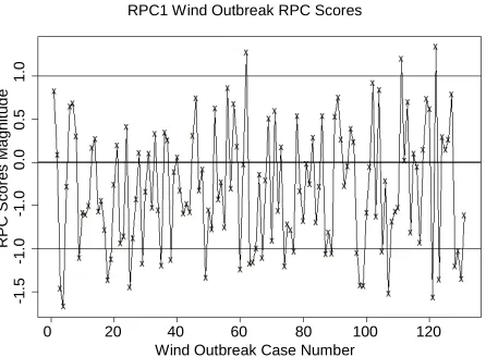
The wind outbreak RPC 1 score plot (Figure 10) shows

that most of the extreme score cases (29% or 22.1%) had

values less than or equal to −1 and only 3 cases (2.3%) had

scores greater than of equal to 1. As the majority of

Tomado Outbreak Case Number RPC1 Tornado Outbreak RPC Scores

0 20 40 60 80

-1

1

2

R

P

C

S

c

or

es

Ma

gni

tud

e

Figure 8. RPC scores for the 79 tornado outbreaks.

Hail Outbreak Case Number RPC1 Hail Outbreak RPC Scores

0 50 100 150 200 250

2

R

P

C

S

c

or

es

Ma

gni

tud

e

1

0

-1

[image:9.595.313.537.369.524.2] [image:9.595.311.534.551.719.2]

(10)

Wind Outbreak Case Number RPC1 Wind Outbreak RPC Scores

0 20 40 60 80 100 120

-1.

5

-1.

0

-1

.0

0.0

0.5

1.0

R

P

C

S

c

or

es

Ma

gni

tud

[image:10.595.63.286.85.249.2]

e

Figure 10. RPC scores for the 131 wind outbreak cases.

the scores are negative, the patterns shown for the load-

ings (Figures 5-7) should have the signs multiplied by

−1 for proper interpretation of those cases associated

with the negative scores.

4. Conclusions

As observation systems generate increasingly dense datasets in space and time, the spatial correlations of the fields can be characterized by the efficient data compression provided by principal component analysis. Until recently, computational power was insufficient to diagonalize the massive data sets of the three-dimensional atmo-

sphere, as currently they are of order 108_{- 10}9_elements

and will increase further to 1010_{elements and greater in}

the near future. The exception has been in situations where the number of cases was relatively small and the analyst was interested in time domain decomposition. We have shown that eigenanalysis of tens of thousands of variables is now achievable. The data reduction achieved in the present analyses diagonalize correlation matrices of order 26,394 dimensions and retain approximately 10 principal components for close to 50% of the variability explained. These principal components are rotated to find the localized coherent variance structures in the data. The RPCs are related to standardized anomalies of the meteorological fields analyzed. Our analyses of the RPC loadings and scores indicate these graphical displays are useful to interpret large datasets in an efficient manner. The results of the rotated PCs for defined outbreak types build upon our previous research [9-12] by indicating that the atmospheric variables investigated exhibit different spatial configurations for each outbreak type.

The challenge is how to use the output of such analyses to improve forecasting of severe weather events. By examining fields of key meteorological variables at lead times (e.g., 24 hours) sufficient to allow for societal re- sponse prior to these outbreaks, we have created a poten-

tially useful product. The next step is to devise a pattern recognition system that compares model predictions of the atmosphere to the patterns produced in this work.

5. Acknowledgements

All of the authors involved in this research were support- ed in part by the National Science Foundation Grant AGS 0831359.

REFERENCES

[1] E. N. Lorenz, “Empirical Orthogonal Functions and Stati- stical Weather Prediction,” Science Report 1, Department of Meteorology, Massachusetts Institute of Technology, 1956.

http://www.o3d.org/abracco/Atlantic/Lorenz1956.pdf [2] J. E. Kutzbach, “Empirical Eigenvectors of Sea-Level

Pressure, Surface Temperature, and Precipitation Com- plexes over North America,” Journal of Applied Meteor- ology, Vol. 6, No. 5, 1967, pp. 791-802.

http://dx.doi.org/10.1175/1520-0450(1967)006<0791:EE OSLP>2.0.CO;2

[3] A. G. Barnston and R. E. Livezey, “Classification, Seaso- nality and Persistence of Low-Frequency Atmospheric Circulation Patterns,” Monthly Weather Review, Vol. 115,

No. 6, 1987, pp. 1083-1126.

http://dx.doi.org/10.1175/1520-0493(1987)115<1083:CS APOL>2.0.CO;2

[4] G. R. North, R. Gerald, T. L. Bell, R. F. Cahalan and F. J. Moeng, “Sampling Errors in the Estimation of Empirical Orthogonal Functions,” Monthly Weather Review, Vol.

110, No. 7, 1982, pp. 699-706.

http://dx.doi.org/10.1175/1520-0493(1982)110<0699:SEI TEO>2.0.CO;2

[5] M. Kim, D. Kim and S. Lee, “Face Recognition Using the Embedded HMM with Second-Order Block-Specific Ob- servations,” Pattern Recognition, Vol. 36, No. 11, 2003,

pp. 2723-2735.

http://dx.doi.org/10.1016/S0031-3203(03)00137-7 [6] H. Moon and P. J. Phillips, “Computational and Perfor-

mance Aspects of PCA-Based Face Recognition Algori- thms,” Perception, Vol. 30, No. 3, 2001, pp. 303-321.

http://dx.doi.org/10.1068/p2896

[7] R. H. Compagnucci and M. B. Richman, “Can Principal Component Analysis Provide Atmospheric Circulation or Teleconnection Patterns?” International Journal of Cli- matology, Vol. 28, No. 6, 2008, pp. 703-726.

http://dx.doi.org/10.1002/joc.1574

[8] G. H. Golub and C. F. Van Loan, “Matrix Computations,” 3rd Edition, John Hopkins, Baltimore, 1996.

[9] A. E. Mercer, C. M. Shafer, C. A. Doswell III, L. M. Le- slie and M. B. Richman, “Objective Classification of Tor- nadic and Nontornadic Severe Weather Outbreaks,” Mon- thly Weather Review, Vol. 137, No. 12, 2009, pp. 4355-

4368. http://dx.doi.org/10.1175/2009MWR2897.1 [10] C. M. Shafer, A. E. Mercer, L. M. Leslie, M. B. Richman

(11)

lations of Tornadic and Nontornadic Outbreaks Occurring in the Spring and Fall,” Monthly Weather Review, Vol. 138, No. 11, 2010, pp. 4098-4119.

http://dx.doi.org/10.1175/2010MWR3269.1

[11] C. M. Shafer, A. E. Mercer, M. B. Richman, L. M. Leslie and C. A. Doswell III, “An Assessment of Areal Cover- age of Severe Weather Parameters for Severe Weather Outbreak Diagnosis,” Weather and Forecasting, Vol. 27,

No. 4, 2012, pp. 809-831.

http://dx.doi.org/10.1175/WAF-D-11-00142.1

[12] A. E. Mercer, C. M. Shafer, C. A. Doswell III, L. M. Le- slie and M. B. Richman, “Synoptic Composites of Torna- dic and Nontornadic Outbreaks,” Monthly Weather Re- view, Vol. 140, No. 8, 2012, pp. 2590-2608.

http://dx.doi.org/10.1175/MWR-D-12-00029.1

[13] C. M. Shafer and C. A. Doswell III, “A Multivariate In- dex for Ranking and Classifying Severe Weather Out- breaks,” Electronic Journal of Severe Storms Meteorol- ogy, Vol. 5, No. 1, 2010, pp. 1-28.

[14] E. Kalnay, M. Kanamitsu, R. Kistler, W. Collins, D. Dea- ven, L. Gandin, M. Iredell, S. Saha, G. White, J. Woollen, Y. Zhu, M. Chelliah, W. Ebisuzaki, W. Higgins, J. Jano- wiak, K. C. Mo, C. Ropelewski, J. Wang, A. Leetmaa, R. Reynolds, R. Jenne and D. Joseph, “The NCEP/NCAR 40-Year Reanalysis Project,” Bulletin of the American Meteorological Society, Vol. 77, No. 3, 1996, pp. 437-

471.

http://dx.doi.org/10.1175/1520-0477(1996)077<0437:TN YRP>2.0.CO;2

[15] R. Swinbank and J. Purser, “Fibonacci Grids: A Novel Approach to Global Modelling,” Quarterly Journal of the Royal Meteorological Society, Vol. 132, No. 619, 2006,

pp. 1769-1793. http://dx.doi.org/10.1256/qj.05.227 [16] M. B. Richman, “Review Paper. Rotation of Principal Com-

ponents,” International Journal of Climatology, Vol. 6,

No. 3, 1986, pp. 293-335.

http://dx.doi.org/10.1002/joc.3370060305

[17] D. S. Wilks, “Statistical Methods in the Atmospheric Sci- ences,” 3rd Edition, Academic Press, Amsterdam, 2011. [18] M. B. Richman and P. J. Lamb, “Climatic Pattern Analy-

sis of 3- and 7-day Summer Rainfall in the Central United States: Some Methodological Considerations and a Re- gionalization,” Journal ofClimate and Applied Meteoro- logy, Vol. 24, No. 12, 1985, pp. 1325-1343.

http://dx.doi.org/10.1175/1520-0450(1985)024<1325:CP AOTA>2.0.CO;2

[19] M. B. Richman and X.-F. Gong, “Relationships between the Definition of the Hyperplane Width to the Fidelity of Principal Component Loading Patterns,” Journal ofCli- mate, Vol. 12, No. 6, 1999, pp. 1557-1576.

http://dx.doi.org/10.1175/1520-0442(1999)012<1557:RB TDOT>2.0.CO;2