Revisting the Rate of Change

Munich Personal RePEc Archive

Revisting the Rate of Change

Khumalo, Bhekuzulu

private research

30 March 2009

Online at

https://mpra.ub.uni-muenchen.de/16014/

Revisiting the Rate of Change Bhekuzulu Khumalo

Abstract:

The Mean Value Theorem is a great theory and guide for any body who deals with the rate of change. This paper aims to add something to the theory. Even a small addition is better than none, only time will tell the significance of the addition.

1.1

It is understood from the Mean Value Theorem that for any polynomial with a degree 2 or higher the derivative is not accurate. Table 1 shows Y = X and the difference, diff, between each x accumulation as well as the derivative. The last column shows the difference in percentage terms of ƒ’(X)/ difference, as can be seen from table 1 ƒ’(X)/ difference in percentage terms is 100%, they are equal, therefore the derivative is equal.

Difference Betw een 'r eal difference' and differentiation of Y = X X X = Y diff ƒ'(X) = 1 %

0 0 n/a 0 N/A

1 1 1 1 100.00

2 2 1 1 100.00

3 3 1 1 100.00

4 4 1 1 100.00

5 5 1 1 100.00

6 6 1 1 100.00

7 7 1 1 100.00

8 8 1 1 100.00

9 9 1 1 100.00

10 10 1 1 100.00 11 11 1 1 100.00 12 12 1 1 100.00 13 13 1 1 100.00 14 14 1 1 100.00 15 15 1 1 100.00 Table 1

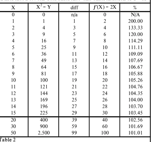
Differ ence Between 'r eal differ ence' and differ entiation of Y = X2 X X2 = Y diff ƒ'(X) = 2X %

0 0 n/a 0 N/A

1 1 1 2 200.00

2 4 3 4 133.33

3 9 5 6 120.00

4 16 7 8 114.29

5 25 9 10 111.11

6 36 11 12 109.09 7 49 13 14 107.69 8 64 15 16 106.67 9 81 17 18 105.88 10 100 19 20 105.26 11 121 21 22 104.76 12 144 23 24 104.35 13 169 25 26 104.00 14 196 27 28 103.70 15 225 29 30 103.45 20 400 39 40 102.56 30 900 59 60 101.69 50 2,500 99 100 101.01 Table 2

Table 2 confirms the derivative will always be higher than the ‘real difference’. As well as the fact that between X = 0, and X = 1, the derivative can greatly exaggerate what the rate of change is and must continuously recover. Therefore as the independent variable gets larger, as expected in ratio terms the derivative gets closer to the ‘real difference’, though in the case of Y = X2, the derivative is always 1 greater than the ‘real difference’.

Differ ence Between 'r eal difference' and differentiation of Y = X3

X X3 = Y diff ƒ'(X) = 3X2 %

0 0 n/a 0 N/A

1 1 1 3 300.00

2 8 7 12 171.43 3 27 19 27 142.11 4 64 37 48 129.73 5 125 61 75 122.95 6 216 91 108 118.68 7 343 127 147 115.75 8 512 169 192 113.61 9 729 217 243 111.98 10 1,000 271 300 110.70 11 1,331 331 363 109.67 12 1,728 397 432 108.82 13 2,197 469 507 108.10 14 2,744 547 588 107.50 15 3,375 631 675 106.97 20 8,000 1,141 1,200 105.17 30 27,000 2,611 2,700 103.41 50 125,000 7,351 7,500 102.03 Table 3

Difference Between 'real difference' and differ entiation of Y = X4

X X4 _{= Y}

diff ƒ'(X) = 4X3

%

0 0 n/a 0 N/A

1 1 1 4 400.00

2 16 15 32 213.33 3 81 65 108 166.15 4 256 175 256 146.29 5 625 369 500 135.50 6 1,296 671 864 128.76 7 2,401 1,105 1,372 124.16 8 4,096 1,695 2,048 120.83 9 6,561 2,465 2,916 118.30 10 10,000 3,439 4,000 116.31 11 14,641 4,641 5,324 114.72 12 20,736 6,095 6,912 113.40 13 28,561 7,825 8,788 112.31 14 38,416 9,855 10,976 111.37 15 50,625 12,209 13,500 110.57 20 160,000 29,679 32,000 107.82 30 810,000 102,719 108,000 105.14 50 6,250,000 485,199 500,000 103.05 Table 4

Differ ence Between 'r eal differ ence' and differ entiation of Y = X5

X X5 _{= Y}

diff ƒ'(X) = 5X4

%

0 0 n/a 0 N/A

1 1 1 5 500.00

2 32 31 80 258.06 3 243 211 405 191.94 4 1,024 781 1,280 163.89 5 3,125 2,101 3,125 148.74 6 7,776 4,651 6,480 139.32 7 16,807 9,031 12,005 132.93 8 32,768 15,961 20,480 128.31 9 59,049 26,281 32,805 124.82 10 100,000 40,951 50,000 122.10 11 161,051 61,051 73,205 119.91 12 248,832 87,781 103,680 118.11 13 371,293 122,461 142,805 116.61 14 537,824 166,531 192,080 115.34 15 759,375 221,551 253,125 114.25 20 3,200,000 723,901 800,000 110.51 30 24,300,000 3,788,851 4,050,000 106.89 50 312,500,000 30,024,751 31,250,000 104.08 Table 5

Now a theory has been established as to why the derivative is always higher, (The Mean Value Theorem), a theory and real prove, the prove being in tables 1 – 5, it is time to correct the mistake and look for a new derivative function that will suite our needs for precision and accuracy.

1.2 Finding the Accurate Function for Rate of Change

Given a function ƒ(X) = aXn (1) Then the derivative ƒ’(X) is:

ƒ’(X) = naXn-1 (2)

We as model builders and social scientist like to be accurate as possible when we can, we want to know the real derivative, ƒ’k(X).

ƒ’k(X) = ƒ’(X) – diff (3)

We can build a general formulae step by step, but first we need to understand why there is a difference between the derivative and the real change, a more compelling reason than merely the tangent, because that will not allow us to extract a real derivative. Take a polynomial say of degree 3, say the function Y = X3. X3 = X X X. Therefore Y = X3 has properties of Y = X2 and Y = X2 in turn has properties that influence it from X. These properties need to be taken out because they are included in the derivative. The larger the polynomial function the more amplified are these properties that need to be taken out. We need to sort of distill the derivative in order to arrive at the real difference, to distill

implies purify. In the case of Y = X3, we need to get rid of the properties from the derivative that defines Y = X2 and Y =X.

One can see this effect if one looks at tables 1 – 5 and by how much percentage points, by how high the ratio is that defines derivative over the real difference. When X = 1, Y = 1, and the derivative is 100% in table 1, 200% in table 2, 300% in table 3, 400% in table 4, and 500% in table 5. Table 1, is when X1, table 2, X2, table 3, X3, table 4, X4 and table 5, X5. One can see the influence gets larger and larger, it is this influence that must be removed, this residual influence of Y = Xn, and the residual influence is equal to Y = Xn-1 as well as the influence of (Xn-2 X1). Obviously the greatest influence would be the preceding

polynomial. (Xn-2 X1) is the residual effect of all the other preceding polynomials without including the immediate preceding polynomial, X1 = X.

Knowing what causes the difference between the derivative and the real derivative we can then attempt to build a general formula for the rate of change, in polynomials, but the conclusions will be universal, for all derivatives. Let us look at Y = X2.

ƒ’k(X) = 2X – 1 (5)

Equation (4) can be the general formula, but it is better to make it look more simple. Not that for Y = X2, the real difference is just the derivative minus 1. That 1 is the real change of Y = X.

It becomes more complex when we move up to the real change of Y = X3. How do we get the real change, the real derivative. We have a guide in equation (4) Therefore we know that:

ƒ’k(X) = ƒ’(X) – ƒ’k(Xn-1) – R that leads to ƒ’k(X) = 3X2 – 2X – R where

3X2 = ƒ’(X) and

2X = ƒ’k(Xn-1) from equation (5)

Now we need to find R the function that defines the residual effects of all the other residual effects.

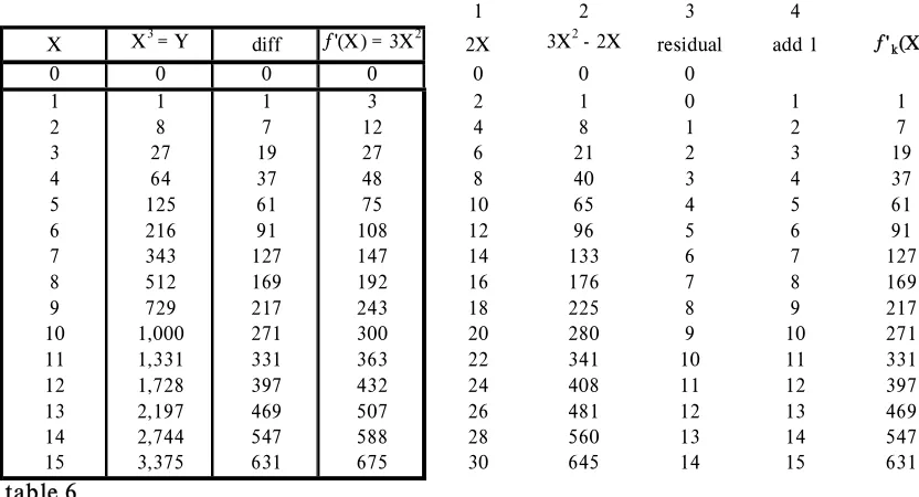
Table 6 is an extension of table 3, it gives us a step by step solution on finding R.

1 2 3 4

X X3 = Y diff ƒ'(X) = 3X2 2X 3X2 - 2X residual add 1 ƒ'k(X)

0 0 0 0 0 0 0

1 1 1 3 2 1 0 1 1

2 8 7 12 4 8 1 2 7

3 27 19 27 6 21 2 3 19

4 64 37 48 8 40 3 4 37

5 125 61 75 10 65 4 5 61

6 216 91 108 12 96 5 6 91

7 343 127 147 14 133 6 7 127

8 512 169 192 16 176 7 8 169

9 729 217 243 18 225 8 9 217

10 1,000 271 300 20 280 9 10 271

11 1,331 331 363 22 341 10 11 331

12 1,728 397 432 24 408 11 12 397

13 2,197 469 507 26 481 12 13 469

14 2,744 547 588 28 560 13 14 547

15 3,375 631 675 30 645 14 15 631

table 6

As mentioned above we first must subtract 2X from 3X2 and we arrive at what is the residual. This is under 3 in table 6. Trying to make sense of the residual we see from table 6 that the residual is 1 less than X. To get a function of the residual one will find that to create a function divisible by X one must always add 1 or subtract 1, in all polynomial functions by taking this action one will find the residual will then be divided by X. Adding 1 to the residual we get X. Therefore when Y = X3, the residual is:

R = (X – 1)

ƒ’k(X) = ƒ’(X) – ƒ’k(Xn-1) – R (4) ƒ’k(X) = 3X2 -2X – (X – 1) (6)

we have to subtract 1 from X because we added 1 in table six in order to get the X in the first place. From equation 6 we get the real derivative for Y = X3:

ƒ’k(X) = 3X2 – 2X – X + 1 and by simplification we get ƒ’k(X) = 3X2 – 3X + 1 (7)

We can test it out to be sure, we can take X = 7 and we get 3(72) – 3(7) + 1

= 147 – 21 +1 = 127 and it is dead on. At one it equals 1.

To clarify our understanding let us take one more example, let us take the polynomial Y = X4.We take guidance from equation (4).

ƒ’k(X) = ƒ’(X) – ƒ’k(Xn-1) – R (4)

Therefore when Y = X4 the real rate of change would be ƒ’k(X) = 4X3 - 3X2 – 3X – R. where

4X3 = ƒ’(X) 3X2 – 3X = ƒ’k(Xn-1)

We now will need to solve for R.

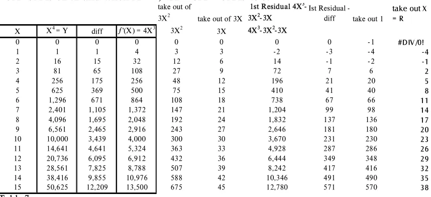
Solving for R, that is to say to see the function that defines the residual we shall take the same route as above, the same route as was used to solve for R to find the real rate of change for Y = X3, the ƒ’k (X3). The process is made easy to understand by including a table to show each step by step process. We include table 7.

In table 7, the first step is to take out the known and be left with R, we therefore find 4X3 – 3X2 – 3X. This value is clearly shown in table 7. When X = 13 from table 7 we see that 4X3 – 3X2 -3X is 8242 and when X = 4, 4X3 – 3X2 – 3X is 196.

take out of

3X2 take out of 3X

1st Residual 4X3

-3X2_{- 3X}

Ist Residual - diff take out 1

take out X = R

X X4 _{= Y}

diff ƒ'(X) = 4X3 _3X2

3X 4X3- 3X2- 3X

0 0 0 0 0 0 0 0 - 1 #DIV /0!

1 1 1 4 3 3 - 2 - 3 - 4 - 4

2 16 15 32 12 6 14 - 1 - 2 - 1

3 81 65 108 27 9 72 7 6 2

4 256 175 256 48 12 196 21 20 5

5 625 369 500 75 15 410 41 40 8

6 1,296 671 864 108 18 738 67 66 11

7 2,401 1,105 1,372 147 21 1,204 99 98 14

8 4,096 1,695 2,048 192 24 1,832 137 136 17

9 6,561 2,465 2,916 243 27 2,646 181 180 20

10 10,000 3,439 4,000 300 30 3,670 231 230 23

11 14,641 4,641 5,324 363 33 4,928 287 286 26

12 20,736 6,095 6,912 432 36 6,444 349 348 29

13 28,561 7,825 8,788 507 39 8,242 417 416 32

14 38,416 9,855 10,976 588 42 10,346 491 490 35

Having arrived at the known solution of 4X3 – 3X2 – 3X we subtract the difference from the original table 4 and we arrive at what is called the 1st residual - diff. The diff being the real difference. Arriving at the solution we subtract 1. As mentioned above at this stage we must always add or subtract 1 in order to have a function that is related to X. At this stage after adding one we find that R at X = 15 is 570 and at say 3 is 6. After taking out 1 we find we can divide by X. The remaining solution follows the function 3X – 7, therefore R for Y = X4 is:

(3X – 7)X + 1. This can be simplified to: 3X2 – 7X + 1

Taking guidance from equation (4)

ƒ’k(X) = ƒ’(X) – ƒ’k(Xn-1) – R (4) we get

ƒ’k(X) = 4X3 – 3X2 – 3X – (3X2 – 7X + 1), this can be simplified to: ƒ’k(X) = 4X3 – 3X2 – 3X – 3X2 + 7X – 1 further simplification: ƒ’k(X) = 4X3 – 6X2 + 4X – 1 (8)

To get real change for Y = X5 the ƒ’k(X) taking guidance from above we get ƒ’k(X) = 5X4 – 4X3 – 6X2 + 4X – R

and we solve for R, not forgetting to add or subtract 1 before solving for R.

1.3 Why Is this Important in Economics

The simple exercise below will show the importance of ƒ’k(X). Take an economic phenomenon Y. This phenomenon is defined as Y = ƒ( A, B, C) (a)

Where A = change in A and A = X3

B = -2X2 C = X

The function for Y is defined as Y = A + B + C (b) Therefore:

Y = (X3) – 2X2 + X (c)

Taking equation (1) from above, recalling equation (2) = ƒ’(X) = naXn-1. Y would be defined as

Y = 3X2 – 2X2 +X (d) which simplified becomes Y = X2 + X (e)

However we understand equation (e) to be wrong because we know that (X3) is not 3X2 but from equation (7) (X3) is = 3X2 – 3X + 1. Therefore the true function of Y is: Y = 3X2 – 3X + 1 – 2X2 + X (f) that when simplified becomes:

Y = X2 – 2X +1 (g)

Conclusion

It is more prudent to use ƒ’k(X), it is correct. Obviously if we had access to a supercomputer we would have solved for every polynomial, but the above is a good enough demonstration. In the symbol ƒ’k(X) the k stands for Khumalo, therefore ƒ’k(X) is known as the Khumalo derivative after the person who discovered it.

Reference:

Khumalo, B. (2009). The Variable Time: Crucial to Understanding Knowledge