Munich Personal RePEc Archive
A Study on Dynamic General
Equilibrium under the Classical Growth
Framework
Li, Wu
29 September 2010
Online at
https://mpra.ub.uni-muenchen.de/25882/
A Study on Dynamic General Equilibrium under the
Classical Growth Framework
Li Wu
Department of Finance, School of Economics, Shanghai University, Shanghai, China [email protected]
Abstract—The equilibrium analyses under the classical growth framework mainly concern production processes so far and the utility-maximization of consumers is not considered sufficiently. Treating a consumer as a producer of labor or land-use right etc. with a utility parameter, this paper presents equilibrium formulas taking account of the utility-maximization of consumers, which may facilitate the analysis of dynamic general equilibrium involving both profit-maximizing firms and utility-maximizing consumers under the classical growth framework. For concreteness, some numerical examples with Cobb-Douglas production and utility functions are utilized to illustrate the method of the equilibrium analysis involving utility-maximizing consumers.
Keywords-dynamic general equilibrium, utility, Sraffian system, von Neumann growth model, land rent
I. INTRODUCTION
The economic table of Quesnay[1], the reproduction model of Marx[2], the input-output modelof Leontief[3,4], the growth model of von Neumann[5] and the equilibrium analysis of Sraffa[6] represent typically the thoughts of classical economics[7,8], and they are essential parts of the classical growth framework. On the basis of the classical growth framework both the dynamic equilibrium analysis and the dynamic disequilibrium analysis can be conducted.
Equilibrium paths under the classical growth framework are usually balanced growth paths, in which supplies of various commodities grow at the same rate. The equilibrium growth rate, the equilibrium price structure and the equilibrium output structure are all determined by technologies (or in other words, production functions) of sectors (or firms). Numerous issues related to equilibrium have been analyzed under the classical growth framework, such as the existence of equilibrium[9], the equilibrium exchange[10], the optimality of equilibrium[11-13], the perturbation of equilibrium[14] and so on. However, such equilibrium analyses mainly concern the production processes so far and the utility-maximization of consumers is not considered sufficiently. In this paper we try to present equilibrium formulas taking account of both profit-maximizing firms and utility-maximizing consumers.
The paper is organized as follows. Section 2 discusses the equilibrium of an economy containing only profit-maximizing firms. Section 3 discusses the equilibrium of an economy containing both profit-maximizing firms and utility-maximizing laborers. Section 4 discusses land rent. Section 5 generalizes the previous equilibrium equations to a von
Neumann-type equilibrium model taking account of the utility-maximization of consumers. Section 6 is devoted to simulations. Section 7 contains some concluding remarks.
II. EQUILIBRIUM EQUATIONS UNDER PROFIT-MAXIMIZING
FIRMS
As the works of Sraffa[6], von Neumann[5]and Hua[15] et al. show, the equilibrium paths under the classical growth framework usually are balanced growth paths. In an economy consisting of n firms producing distinct commodities with Leontief production functions, when an indecomposable nonnegative input coefficient matrix A is given an equilibrium output vector y*
must be a right P-F (i.e. Perron-Frobenius)
eigenvector of A, and an equilibrium price vector p* must be a left P-F eigenvector of A[15]. The equilibrium growth rate is
1 1
wherein is the P-F eigenvalue of A. That is, the following equilibrium equations hold:
* 1 *
1
T T
p A p
* 1 *
1
Ay y
We will refer to (1) as the price equilibrium equation and refer to (2) as the output equilibrium equation.
Until now the equilibrium analyses under the classical growth framework focus mainly on production processes and it seems that the utility-maximization of consumers hasn’t been considered sufficiently. In what follows we will show that the equilibrium equations above can be extended to deal with the utility-maximizing consumers as well when we treat a consumer as a producer of labor or land-use right etc. with a utility parameter. For concreteness, some numerical examples with CD production and utility functions will be utilized to illustrate the method of the equilibrium analysis involving utility-maximizing consumers.
First let’s extend (1) and (2) to deal with the equilibrium of an economy containing profit-maximizing firms with non-Leontief production functions.
0.6 0.1 0.3 1 2 3
5x x x , 3x x x10.4 0.42 30.2 and
0.2 0.7 0.1 1 2 3
x x x respectively. All these functions are homogeneous of degree one, that is, constant returns to scale hold.
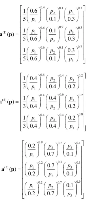
In this case the input coefficient matrix can be treated as a function of the price vector [16]. Given a price vector p, the input amounts (i.e. the input bundle) needed by each profit-maximizing firm to produce one unit of commodity can be computed. The input bundles of 3 firms constitute the following input coefficient matrix:
(1) (2) (3)
( ) ( ) ( ) ( )
A p a p a p a p
wherein a(1)( )p , a(2)( )p and a(3)( )p are as follows:
0.4 0.1 0.3 3 2
1
0.9 0.3 0.6
(1) 1 3
2 0.7 0.6 0.1 1 2 3 1 0.6
5 0.1 0.3
1 0.1
( )
5 0.6 0.3
1 0.3
5 0.6 0.1
p p p p p p p p p
a p
0.6 0.4 0.2 3 2
1
0.6 0.2 0.4
(2) 1 3
2 0.8 0.4 0.4 1 2 3 1 0.4
3 0.4 0.2
1 0.4
( )
3 0.4 0.2
1 0.2
3 0.4 0.4
p p p p p p p p p
a p
0.8 0.7 0.1 3 2
1
0.3 0.1 0.2
(3) 1 3
2 0.9 0.2 0.7 1 2 3 0.2 0.7 0.1 0.7 ( ) 0.2 0.1 0.1 0.2 0.7 p p p p p p p p p
a p
Let p* and y* denote respectively an equilibrium price vector and an equilibrium output vector in an equilibrium path, then the equilibrium input coefficient matrix is *
( )
A p . p*
and *
y must be a left P-F eigenvector and a right P-F eigenvector of *
( )
A p respectively, hence we have the following equilibrium equations:
* * 1 *
( ) 1 T T
p A p p
* * 1 *
( )
1
A p y y
By solving the price equilibrium equation (7), the unique normalized equilibrium price vector is computed to be
*
(0.1231, 0.2535, 0.6234)T
p , and the equilibrium growth rate is computed to be 16.49% , which is the maximal balanced growth rate in this economy.
[image:3.595.88.267.241.592.2]Suppose the initial supply amount of commodity 3 is 100 units. By solving the output equilibrium equation (8) the initial production processes in the equilibrium path turn out to be:
TABLE I. INPUT-OUTPUT PROCESSES
Firm 1 Firm 2 Firm 3 Total Inputs
Comm. 1 Inputs 607.72 303.86 101.29 1012.9
Comm. 2 Inputs 49.19 147.57 172.17 368.93
Comm. 3 Inputs 60 30 10 100
Outputs 1179.8 429.75 116.49
Among various methods of solving (7), a simple one is to resort to an iteration function ( 1) ( )
G( )
k k
p p , in which p(k1) is the normalized left P-F eigenvector of ( )
( k )
A p . It’s not difficult to prove the convergence of this iteration function on the basis of Lyapunov’s second method[17] by investigating the P-F eigenvalue of ( )
( k )
A p .
III. EQUILIBRIUM EQUATIONS UNDER PROFIT-MAXIMIZING
FIRMS AND UTILITY-MAXIMIZING LABORERS
Now let’s replace firm 3 of the economy in Section 2 by some homogeneous utility-maximizing laborers, and then study the equilibrium of the economy containing both profit-maximizing firms and utility-profit-maximizing laborers.
Suppose the production functions of firm 1 and firm 2 are still 5x x x10.6 20.1 30.3 and
0.4 0.4 0.2 1 2 3
3x x x , the utility function of each laborer is x x x10.2 0.72 30.1, and each laborer supplies one unit of labor (i.e. commodity 3) in each period.
In this case the input coefficient matrix can be treated as a function of the price vector p and the utility level . The input coefficient matrix in this example may be written
(1) (2) (3)
( , ) ( ) ( ) ( )
A p a p a p a p
wherein (1) ( )
a p , (2) ( )
a p and (3) ( )
a p are indicated by (4)-(6).
unit of output and the inputs that a utility-maximizing laborer needs to obtain units of utility under the price vector p.
Suppose the population of laborers and the supply amount of labor grow at an exogenous rate ( 1, ), then the equilibrium growth rate must be if there exists an equilibrium. In an equilibrium path the price vector and the utility level of laborers keep constant, while the outputs of firms and the supply of labor grow at the same rate. Hence in an equilibrium path the laborers can be regarded as the “producer” of labor with an equilibrium utility level *, and the last column of the input coefficient matrix is the input bundle needed to produce one unit of labor.
Let p* and y* denote respectively an equilibrium price vector and an equilibrium output vector in an equilibrium path. Then * *
( , )
A p is the equilibrium input coefficient matrix. Now we have the following equilibrium equations:
* * * 1 *
( , )
1
T T
p A p p
* * * 1 *
( , )
1
A p y y
By solving the price equilibrium equation (10) we can obtain the equilibrium price vectors p* and the equilibrium utility level *
.
When the supply of labor keeps constant all the time (i.e.
0
), the unique normalized equilibrium price vector is computed to be p* (0.0866, 0.1652, 0.7482)T . And the equilibrium utility level is *1.9872. The corresponding equilibrium input coefficient matrix is
* *
0.6 0.7631 1.7279
( , ) 0.0524 0.4 3.1699
0.0347 0.0442 0.1
A p
Suppose further the supply of labor is 100 units all the time, by solving the output equilibrium equation (11) we find the production and consumption processes in the equilibrium path are as follows:
TABLE II. INPUT-OUTPUT PROCESSES (0)
Firm 1 Firm 2 Laborers Total Inputs
Comm. 1 Inputs 1036.7 518.36 172.79 1727.9
Comm. 2 Inputs 90.568 271.7 316.99 679.26
Labor Inputs 60 30 10 100
Outputs 1727.9 679.26 100
The consumption bundle of each laborer is (1.7279, 3.1699, 0.1)T
.
When the supply of labor grows at an exogenous growth rate 5% per period (i.e. 0.05 ), by solving the price equilibrium equation (10) we find the unique normalized equilibrium price vector is p* (0.0977, 0.1909, 0.7114)T and the equilibrium utility level is *
1.5954
.
If the initial supply of labor is 100 units, by solving the output equilibrium equation (11) we find the production and consumption processes in the equilibrium path are as follows:
TABLE III. INPUT-OUTPUT PROCESSES (0.05)
Firm 1 Firm 2 Laborers Total Inputs
Comm. 1 Inputs 873.97 436.99 145.66 1456.6
Comm. 2 Inputs 74.511 223.53 260.79 558.83
Labor Inputs 60 30 10 100
Outputs 1529.5 586.77 105
The consumption bundle of each laborer is
(1.3873, 2.4837, 0.0952)T
. The vector (1456.6, 558.83, 100)T
is referred to as an equilibrium input vector.
The price equilibrium equation (10) can also be solved by an iteration function ( 1) ( )
G ( )
k k
p p . Given p( )k
, p(k1) is computed through the following steps: firstly find a positive real number ( )k
such that the P-F eigenvalue of ( ) ( ) ( k ,k )
A p
equals 1 (1), then let p(k1)
be the normalized left P-F eigenvector of ( ) ( )
( k,k )
A p . The convergence of this iteration function can be proved on the basis of Lyapunov’s second method[17] by investigating ( )k .
Now let’s discuss the amount ratios of the same kind of inputs used by distinct agents in equilibrium.
Let pˆ denote the diagonal matrix with the vector p as its
main diagonal. Let v* p x* *
denote the equilibrium input value vector, i.e. the equilibrium input vector measured in currency, in which *
p and *
x arethe equilibrium price vector and the equilibrium input vector (measured in physical unit) respectively.
The exponents of agents’ CD production and utility functions constitute the following matrix C:
0.6 0.4 0.2
0.1 0.4 0.7
0.3 0.2 0.1
C
vectors), it’s easy to know *
v must be a right P-F eigenvector
of the matrix C and each row of Cv*
indicates the amount ratios of the same kind of inputs used by distinct agents in equilibrium. For example, a right P-F eigenvector of the matrix
C in (13) is *
(4, 3, 2)T
v , and
*
2.4 1.2 0.4
0.4 1.2 1.4
1.2 0.6 0.2
Cv
The third row of Cv*
indicates the amount ratios of labor used by distinct agents in equilibrium are 1.2:0.6:0.2, i.e. 6:3:1.
IV. LAND RENT
Besides labor, the supply amounts of some other commodities such as land (or land-use right), mineral deposits etc. may also be exogenous, and land may be taken as a representative.
The theory of land rent has been discussed by a number of authors [18-23]. Assuming simply that land is uniform in quality, here we attempt to explore a new method of computing the equilibrium land rent, that is, we’ll compute the equilibrium land rent by the equilibrium equations taking account of the utility-maximization of landowners.
Now let’s suppose there are a firm, some homogeneous landowners and some homogeneous laborers in the economy. Suppose the production functions of the firm is 5x x x10.6 20.1 30.3, the utility function of each landowner is 0.4 0.4 0.2
1 2 3
3x x x , and the utility function of each laborer is 0.2 0.7 0.1
1 2 3
x x x . Each landowner
supplies a unit of land-use right (or loosely speaking, land) per period. With a unit of land-use right, an agent may use a unit of land for one period. The price of a unit of land-use right is referred to as land rent.
Now the input coefficient matrix is
(1) (2) (3)
1 2 2 1
( , , ) ( ) ( ) ( )
A p a p a p a p
Columns of the input coefficient matrix A p( , 1, 2)
indicate the inputs that a profit-maximizing firm needs to obtain one unit of output and the inputs that a utility-maximizing laborer (or landowner) needs to obtain 1 (or 2) units of utility under the price vector p.
Suppose the supplies of labor and land grow at an exogenous rate . Then the equilibrium growth rate must be if there is an equilibrium. And we have the following equilibrium equations:
* * * * *
1 2
1
( , , )
1
T T
p A p p
* * * * *
1 2
1
( , , )
1
A p y y
Now we cannot find the equilibrium price vectors only by the price equilibrium equation (16). That is, to compute the equilibrium prices now we also need the output equilibrium equation (17). In addition, in the example here we need to know the supply ratio y2* y3* (i.e. the supply ratio of land to labor).
Suppose the supply of land is 60 units all the time, and the supply of labor is 100 units all the time, that is, y*2 60 and
* 3 100
y . Then the unique normalized equilibrium price vector
is computed to be *
(0.0572, 0.6734, 0.2694)T
p .
Note that the ratio between the equilibrium total values of land and labor is 3/2, and the supply amounts of land and labor are 60 units and 100 units respectively, hence the equilibrium ratio between land rent and labor price (i.e. wage rate) must be
3 2 60 100
, i.e. 2.5, which is independent of the exogenous growth rate .
The production and consumption processes in the equilibrium path are as follows:
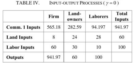
TABLE IV. INPUT-OUTPUT PROCESSES (0)
Firm Land-
owners Laborers Total Inputs
Comm. 1 Inputs 565.18 282.59 94.197 941.97
Land Inputs 8 24 28 60
Labor Inputs 60 30 10 100
Outputs 941.97 60 100
When the utility function of each landowner is x x x10.2 20.7 30.1 instead of 3x x x10.4 0.42 30.2 and other conditions keep unchanged, the unique normalized equilibrium price vector is computed to be *
(0.0404, 0.7997, 0.1599)T
p , hence we see that the
equilibrium price vector is related to the utility function of landowners. Now the equilibrium ratio between land rent and labor price is 5.
[image:5.595.323.541.359.461.2]The production and consumption processes in the equilibrium path are as follows:
TABLE V. INPUT-OUTPUT PROCESSES (0)
Firm Land-
owners Laborers Total Inputs
Comm. 1 Inputs 475.26 237.63 79.21 792.1
Land Inputs 4 42 14 60
Labor Inputs 60 30 10 100
Now let’s return to the original example and suppose the exogenous growth rate is 5%, then the unique normalized equilibrium price vector is computed to be
*
(0.0641, 0.6685, 0.2674)T
p . And the initial production and consumption processes in the equilibrium path are as follows:
TABLE VI. INPUT-OUTPUT PROCESSES (0.05)
Firm Land-
owners Laborers Total Inputs
Comm. 1 Inputs 500.28 250.14 83.381 833.81
Land Inputs 8 24 28 60
Labor Inputs 60 30 10 100
Outputs 875.5 63 105
V. A VON NEUMANN-TYPE EQUILIBRIUM MODEL WITH
CONSUMPTION AND UTILITY-MAXIMIZATION
As the traditional von Neumann-type equilibrium models show, when joint production is taken into account the equilibrium formulas will be inequalities instead of equations, and there will be an output coefficient matrix B in addition to an input coefficient matrix A[5, 9, 19]. Moreover, A and B may be non-square matrices. The output vector y will also be substituted by a semipositive activity level vector z.
In order to build a von Neumann-type equilibrium model with consumption and utility-maximization, here we shall:
(i) Treat the input and output coefficient matrices A and B
as functions (sometimes multivalued functions) of the semipositive price vector p and utilities. Now a column of A
and a corresponding column of B usually stand for technologies of a firm or some homogeneous consumers rather than a single technology as in the traditional von Neumann-type equilibrium models.
(ii) Treat the consumption processes of laborers and landowners et al. in a manner formally analogous to the production processes of firms, that is, treat a consumer as a producer of labor or land-use right etc. with a utility parameter. And some components of the activity level vector z will be exogenous to stand for the exogenous supply amounts of labor and land etc.
(iii) Assume that the supplies of labor and all types of land grow at an exogenous rate , and labor is always indispensable for the economy. Since technology progress is excluded and all profits are assumed to be put into reproduction, the equilibrium growth rate and the equilibrium profit rate must equal the exogenous supply growth rate of labor.
For simplicity, here let’s make the following assumptions:
(i) Labor is homogeneous, and each laborer supplies one unit of labor per period. All laborers have the same degree one homogeneous utility function.
(ii) There are k types of land, and each landowner owns only one type and one unit of land. All landowners of the same
type of land have the same degree one homogeneous utility function.
(iii) Labor is indispensable for the production of each commodity with endogenous supply, and each non-zero consumption bundle of laborers and landowners contains at least one kind of commodity with endogenous supply.
Now the utility of each laborer (i.e. 1) and the utilities of landowners (i.e. 2,,k1) constitute a utility vector υ. Let
denotes the subsistence utility level of laborers. Let denote the wage rate, which is a component of p. Then we have the following von Neumann-type equilibrium model:
* * * 1 * * *
( , ) ( , )
1
T T
p A p υ p B p υ
* * * 1 * * *
( , ) ( , )
1
A p υ z B p υ z
* * * * 1 * * * *
( , ) ( , )
1
T T
p A p υ z p B p υ z
*
1 0
*
0
(18) and (19) imply (20), and (20) may be omitted[9].
Here let’s simply illustrate the model above by two numerical examples.
First let’s look at a Leontief-type numerical example.
Suppose there are 5 commodities, i.e. a commodity with endogenous supply, labor and 3 types of land. All laborers and landowners have the same Leontief utility functions (see the following input coefficient matrix). There are 3 firms producing the same commodity with distinct Leontief production functions. The supply of labor is 150 units all the time. The supply of each type of land is 60 units all the time. That is, 0 and ( , ,1 2 3, 150, 60, 60, 60)
T
z z z
z . Let be
0.1. The input and output coefficient matrices are
1 2 3 4
1 2 3 4
0.3 0.6 0.8 0.3 0.3 0.3 0.3
0.1 0.2 0.4 0.1 0.1 0.1 0.1
( ) 0.2 0 0 0 0 0 0
0 0.4 0 0 0 0
A υ
0 0 0 0.6 0 0 0 0
1 1 1 0 0 0 0 0 0 0 1 0 0 0 0 0 0 0 1 0 0 0 0 0 0 0 1 0 0 0 0 0 0 0 1
There are multiple normalized equilibrium price vectors in this example. A normalized equilibrium price vector is
*
(0.1818, 0.1222, 0.5753, 0.1207, 0)T
p . The corresponding
equilibrium utility vector is υ*(1.8301, 8.6166, 1.8083, 0)T. And the unique equilibrium activity level vector is
*
(300, 150, 0, 150, 60, 60, 60)T
z .
If the supply of labor is 300 units instead of 150 units, by computation we see that labor is in excess supply. That is, both the “equilibrium” wage rate and “equilibrium” utility level of each laborer equal 0, or in other words, there is no equilibrium according to our definition.
Next let’s look at a Cobb-Douglas-type numerical example.
Suppose there are 4 commodities, i.e. a commodity with endogenous supply, labor and 2 types of land. All laborers and landowners have the same CD utility functions 0.2 0.7 0.1
1 2 3 x x x . There are 2 firms producing the same commodity with distinct CD production functions, i.e. 5x x x10.6 20.1 30.3 and
0.6 0.1 0.3 1 2 4
3x x x
respectively. The supply of labor is 150 units all the time. The supply of each type of land is 60 units all the time. That is,
0
and ( , , 150, 60, 60)1 2
T
z z
z . Let be 0.1. Here let’s assume that the price vector is positive. The input coefficient matrix can be computed on the basis of the production and utility functions. The output coefficient matrix is
1 1 0 0 0 0 0 1 0 0 0 0 0 1 0 0 0 0 0 1
B
The computation results are as follows.
The unique positive normalized equilibrium price vector is *
(0.0662, 0.5094, 0.3591, 0.0654)T
p . The corresponding
equilibrium utility vector is υ* (0.6986, 0.4925, 0.0897)T , and the corresponding equilibrium activity level vector is
*
(572.1, 197.7, 150, 60, 60)T
z . The equilibrium input
coefficient matrix is
*
0.6 0.6 1.5396 1.0853 0.1977 0.0130 0.0130 0.7 0.4934 0.0899
( , )
0.0553 0 0.1419 0.1 0.0182 0 0.3035 0 0 0
*
A p υ
Analogous to the equilibrium equations (7) and (8), when consumption is excluded the utility vector υ and (21) will disappear from the model, and will become endogenous.
VI. SIMULATIONS
In this section let’s use a structural growth model, i.e. the model (19a)-(19c) in [24], to simulate the dynamics of the
economy with 0 growth rate in Section 3, in which the supply of labor is 100 units all the time. Here we use the following price adjustment function instead of the original one:
( 1) ( ) ( )
0.7+0.3
t t t
p u p
Now the input coefficient matrix in the model is A p( , ) , and the value of may be computed after each exchange process. Note that the value of doesn’t affect the exchange process in essence, that is, it doesn’t affect the purchase and sales bundles of each agent, hence may be always set to 1 in an exchange process.
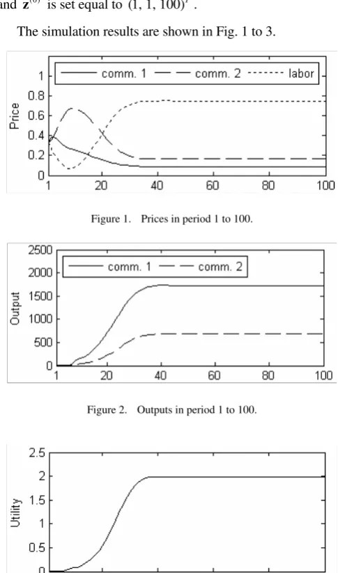
The initial values p(0) and u(0) are set equal to (1, 1, 1)T, and z(0)
is set equal to (1, 1, 100)T
.
[image:7.595.309.552.232.644.2]The simulation results are shown in Fig. 1 to 3.
[image:7.595.54.289.556.616.2]Figure 1. Prices in period 1 to 100.
Figure 2. Outputs in period 1 to 100.
Figure 3. Utility of each laborer in period 1 to 100.
Recall that the normalized equilibrium price vector is
prices of all commodities converge to the normalized equilibrium prices.
Recall that the equilibrium output vector is *
(1727.9, 679.26, 100)T
y , Fig. 2 shows that the outputs of commodity 1 and commodity 2 converge to the equilibrium output levels.
Fig. 3 shows that the utility of each laborer converges to the equilibrium utility level 1.9872.
For other Cobb-Douglas-type numerical examples in this paper the simulation results are similar.
VII. CONCLUDING REMARKS
For dynamic economic models, equilibrium is usually defined as a special kind of paths, e.g. the balanced growth paths with the maximal growth rate or the paths with ever-clearing markets. In various economic models different conditions are utilized to define equilibrium, and the equilibria defined by different conditions may correspond to the similar path sets or the same path set (e.g. the balanced growth path set). The equilibria investigated by Sraffa are essentially balanced growth paths[6]. In the von Neumann growth model the equilibrium conditions differ from those of Sraffa, but the equilibria are also balanced growth paths[5].
Centering on balanced growth paths, the equilibrium analyses under the classical growth framework mainly concern production processes so far and the utility-maximization of consumers is not considered sufficiently. Treating a consumer as a producer with a utility parameter, this paper presents equilibrium formulas taking account of the utility-maximization of consumers, which may facilitate the analysis of dynamic general equilibrium involving both profit-maximizing firms and utility-profit-maximizing consumers under the classical growth framework.
REFERENCES
[1] Quesnay, F. Quesnay's Tableau Economique [1759]. Edited by M. Kuczynski and R. L. Meek. London: Macmillan, 1972.
[2] Marx, K. Capital, vol. II, English translation of Das Kapital, vol. II, edited by F. Engels (Hamburg, Meissner, 1885). Moscow: Progress Publishers, 1956.
[3] Leontief, W. “Quantitative Input-Output Relations in the Economic System of the United States”, Review of Economics and Statistics, 18, pp. 105-125, 1936.
[4] Leontief, W. Structure of the American Economy, 1919-1929. Cambridge, Mass.: Harvard University Press, 1941.
[5] von Neumann, J. “A Model of General Economic Equilibrium”, Review of Economic Studies, 13, pp. 1–9, 1945.
[6] Sraffa, P. Production of Commodities by Means of Commodities. Cambridge: Cambridge University Press, 1960.
[7] Kurz, H. and N. Salvadori. “‘Classical’ Roots of Input-Output Analysis: A Short Account of its Long Prehistory”, Economic Systems Research, 12(2), pp. 153-179, 2000.
[8] Kurz, H. and N. Salvadori. “Sraffa and von Neumann”, Review of Political Economy, 13(2), pp. 161-180, 2001.
[9] Kemeny, J. G., O. Morgenstern and G. L. Thompson. “A Generalization of the von Neumann Model of an Expanding Economy”, Econometrica, 24, pp. 115-135, 1956.
[10] Gale, D. The Theory of Linear Economic Models. New York: McGraw-Hill, 1960.
[11] Dorfman, R., P. A. Samuelson and R. M. Solow. Linear Programming and Economic Analysis. New York: McGraw-Hill, 1958.
[12] McKenzie, L. W. “Turnpike Theorems for a Generalized Leontief Model”, Econometrica, 31, pp. 165-180, 1963.
[13] McKenzie, L. W. “Turnpike Theory”, Econometrica, 44, pp. 841-865, 1976.
[14] Dietzenbacher, E. “Perturbations of Matrices: A Theorem on the Perron Vector and its Applications to Input-output Models”, Journal of Economics, 48(4), pp. 389-412, 1988.
[15] Hua, L. “On the Mathematical Theory of Globally Optimal Planned Economic Systems”, Proceedings of the National Academy of Sciences of the United States of America, 81, pp. 6549-6553, 1984.
[16] Zhang, Jinshui. “A Multi-sector Nonlinear Dynamic Input-Output Model with Human Capital”, Economic Systems Research, 20(2), pp. 223-237, 2008.
[17] Luenberger, D. Introduction to Dynamic Systems: Theory, Models, and Applications. John Wiley&Sons, 1979.
[18] Bidard, C. Prices, Reproduction, Scarcity, Cambridge: Cambridge University Press, 2004.
[19] Bidard, C. “General Theory of Rent”. Presented at the International Conference on Production and Distribution, Meiji University, Tokyo, Sept., 2010.
[20] Kurz, H. “Rent Theory in a Multisectoral Model”, Oxford Economic Papers, 30(1), pp. 16-37, 1978.
[21] Salvadori, N. “Land and Choice of Techniques within the Sraffa Framework”, Australian Economic Papers, 25, pp. 94-105, 1986. [22] Schefold, B. Mr. Sraffa on Joint Production and Other Essays. London:
Unwin & Hyman, 1989.
[23] Woods, J. “A Note on Rent”, Oxford Economic Papers, 39, pp. 388-411, 1987.