Munich Personal RePEc Archive
Does trading remove or bring frictions?
Lin, William and Sun, David and Tsai, Shih-Chuan
Kai Nan University
August 2010
Online at
https://mpra.ub.uni-muenchen.de/37285/
Does Trading Remove or Bring Frictions?
William T. Lin Tamkang University
David S. Suna
Kainan University
Shih-Chuan Tsaib
National Taiwan Normal University
(For the special issue of EMFT)
a
Address correspondences to: David Sun, Kainan University, PO Box 11061, Taipei, Taiwan 100, or davidsun0769@gmail.com
b
Abstract
We explore in this paper how trading noise, when considered as a market friction, reacts to trading activity. Transactions cost is a good explanation for intraday trading behavior in the market according to our data. Particularly, we show that in general trading brings friction to market. However, trading friction at market open is the lowest during the day, as trading causes less friction then relatively. This is due to the behavioral difference among investors. When market opens, individual trading removes, while institutional trading brings, market friction. Situation in the rest of the day is just the opposite, where individual, instead of institutional, trading brings friction. The uneven behavior of trading noise across investors and time of day makes it a specific, rather than general, transactions cost, as opposed to Stoll (2000). Intraday trading activity suppresses both order width and depth, as proxies for trading intensity, therefore creates more noise or friction in the market. Width and depth contribute to trading noise in a polarized way, so that individual trading hurts friction in small cap stocks at open, but benefits it at close. Institutional trading brings extremely strong friction to large cap stocks, but less so at market close. So trading noise as a specific, rather than general, transactions cost is prominent only to certain investors, at certain time and for certain stocks in the market. Our findings lend itself to the justification of the new financial transactions tax proposed by the European Union.
Keywords: Noise, transaction cost, herding, search model, order book
I. Introduction
Trading in markets involves general transaction costs applicable to the entire market as well as
specific costs only born by certain investors. The former acts as a friction in trading, which could be
noises as argued in Stoll (2000) or herding out of information cascades (see Nofsinger and Sias
(1999), Banerjee (1992), Bikhchandani, Hirshleifer, and Welch (1992) and Avery and Zemsky
(1999, AZ), among others). The latter could also take the form of information asymmetry (as
discussed in Diamond and Verrecchia (1981), Glosten and Milgrom (1985), Kyle (1985), Admati
(1991), Easley and O’Hara (1992) and Easley, Kiefer, and O’Hara (1997)). This study addresses the
role of trading noise as a friction to market participants, especially in the presence of trading
concentration. Our interest is in whether trading activity itself adds to or drives down this friction,
and how the relationship is affected by investor type, market capitalization of stocks and time of
day the trading takes place. If trading brings friction, then our findings provide support to financial
transactions tax which encounters much resistance.
We attempt to verify in this study if trading noise really qualifies to be a general transactions
cost, or a market-wide friction, in an intraday framework. It has been well documented in Amihud
and Mendelson (1987), Stoll and Whaley (1990), and Stoll (2000) that stock return volatility is the
highest right after market opens. Stoll (2000) suggests that the high volatility is caused by friction, a
general transaction cost for everyone in the market. Alternatively, Lakonishok, Shleifer, and Vishny
(1992, LSV) and Wermers (1999) stress that volatility is closely related to information-induced
herding behavior. However, Lin, Tsai and Sun (2011) argue that comparative advantage in search
cost dictates a polarization of trading activity across investors, firm size and time of day. Based on
that notion, an investor can optimize by allocating trades when transaction cost is the most
favorable. Hu (2006) applied a return decomposition mechanism to conclude that specific
transactions cost causes the market to be the most volatile at open since frictional noises are the
smallest during the day. We adopt this concept but attempt to identify its driving factors.
We find in this study that trading activity brings friction to market. However, friction at market
open tends to be the lowest during the day, as trading causes less friction relatively at that time. This
is due to the behavioral difference among investors. When market opens, individual trading
removes, while institutional trading brings, market friction. Situation in the rest of the day is just the
opposite, where individual, instead of institutional, trading brings friction. The uneven behavior
pattern of trading noise across investors and time of day makes it a specific, rather than general,
is stronger when trading is more concentrated, different from the prediction of Lin, Sanger, and
Booth (1995) and Hu (2006). Although in general the time needed to fill an order, or the inverse of
the number of orders matched with a certain time window, is inversely related to trading noise, it is
quite the contrary at market open. Moreover, we argue that noise is influenced more by trading
concentration, at open than at close. We also find that market width of limit order book, which
measures how tightly the orders are placed to each other or how closely they are to the mid-quote, affect
trading noise. Market depth exhibits similar influence. Response of noise to market width and depth
differs by market capitalizations as well as by trading hours. Individual trading aggravates at open, but
benefits at close, friction in the trading of small cap stocks. Despite that institutional trading brings
extremely strong friction to large cap trading, it still contributes relatively less to trading friction at
market close.
We consider in this study trading intensity more in a dynamic sense by measuring order
intensity rather than quantity, with sequences of buy or sell runs based on Patterson and Sharma
(2006, PS). It captures intraday order flows better than the popular LSV method, which is more
suitable for longer time frame. The dynamic trading intensity helps us capturing how ‘friction’
really arises from trades. Although noise proportion of stock returns is high on individual orders
and low on institutional orders, its behavior at market open is entirely different from the rest of the
day. Noises for small cap stocks, unlike volatilities, are lower than those for large cap stocks. For
individuals, noise benefits trading stocks of smaller firms, while for institutional investors it its
market width and depth that benefit trading stocks of larger firms. This distinct pattern of trading
activity is not compatible with information-based explanation, especially why market width is lower,
at market open, when trading is extremely heavy. Institutionals prefer to trade large cap stocks,
especially at market close, while individuals are more eager to trade small caps at market open. So
trading noise is just a specific transaction cost, as information cost, prominent only to certain
investors in the market. If trading noise is not compatible with general market phenomena, then it
may not be a general transaction cost as argued in Stoll (2000). Trading noise is just another kind of
specific cost, rather than a market-wide friction.
As we find trading brings friction, our findings provide support to the new financial
transactions tax proposed by the European Union, which has invited lots of criticism. The results of
this study also indicate that uneven trading noise makes market trading polarized. Transactions cost,
rather than information dissemination, is the more important factor causing the result. Our study
also helps identifying for various types of investors a more cost-efficient time to trade. Both
trading. But foreign institutional benefit more from trading at market close than at market open
when trading does not concentrate. A brief literature review and discussion is given in Section II.
Data and empirical results are laid out in Section III. Conclusion is given in Section IV.
II. Noise and Trading
Trading noise has long been considered a crucial factor to asset returns. When market trading
is more heavily concentrated, noise plays a more important role. Literature has modeled noise as
investor irrationality or information barrier, among others. Although the direct effect of noise
trading to a securities market seems to be reducing informational efficiency, there are views on the
positive side of noise. Greater noise trading induces rational agents to trade more aggressively on
their existing information and provides them with incentives to acquire better information. As a
result, Grossman and Stiglitz (1980) and Kyle (1985), argue that noise trading does not reduce
informational efficiency. Furthermore, Kyle (1985) suggests that noise trading improves
informational efficiency.
Various models consider rational agents not being able to fully offset noise traders’ demands
because of limits to arbitrage. De Long, Shleifer, Summers, and Waldmann (1990) indicate that
rational arbitrageurs may magnify demand shocks from noise traders because anticipated worsening
mispricing in the short-run. Relative to the issue of trading noise, Bikhchandani and Sharma (2001)
classify herding behavior into rational and irrational ones. Rational herding takes place when
investors make the same response to a piece of information or when they exhibit similar preference
for a stock, while irrational herding occurs as investors ignore their own information but imitate or
follow others’ trades. These views are not compatible with how noise trading is modeled.
Other than Kyle (1985), many have also studied trading against one's own private information
(e.g., Jarrow (1992), Chakraborty and Yilmaz (2004)) in market manipulation, where the informed
may trade in a wrong direction to increase noise in trading volume. Herding behavior is also
considered a challenge to the efficient market paradigm. At a group level it is considered irrational
as it leads to mispricing, but it can be rational at an individual level. Literature argues that the
herding arises from agents copying one another in trading decisions. The models of BHW and
Bannerjee (1992) consider that individuals make their decisions sequentially at a time, taking into
account the decisions of the individuals preceding them. The model proposed by Cont and
Bouchaud (2000) consider, instead of a sequential decision process, a random communication
structure. Random interactions among agents lead to a heterogeneous market structure. AZ argues,
one contrarian trade from the herd can quickly stop an information cascade.
Noise and Information
Following the definition of Hu (2006), we make the following decomposition of the log price
of a given stock,
t t
t m n
P = + , Et[nt+j]=0, and Et[ntnt+j]=0as j→∞ (1)
where mt is considered as the permanent component of the stock price and follows a random walk
process,
t t
t m u
m = −1+ , Et−1[ut]=0,
2 2
]
[ut u
E =σ , and E[utnt−i]=0, i=1,2,… (2)
Where ut is a white noise and is orthogonal to mt−1. The other component of Pt, nt, is a
temporary noise which disappears over time. After simple algebra, we would obtain
t j t t
t P P n
E[ − + ]= as j→∞
The volatility of stock return Var(Pt−Pt−1) can be decomposed into Var(ut), Var(nt−nt−1) and
) ,
(ut nt−nt−1
Cov . The ratio
) (
) (
1 1
− −
− − =
t t
t t t
P P Var
n n Var
N (3)
will be used as a relative measure of noise within stock return volatility subsequently. When noise
ratio of the entire market is computed, transactions price is used. But the midpoint of buy and sell
order price is used in place of market price when noise ratio of a certain type of investor is to be
computed.
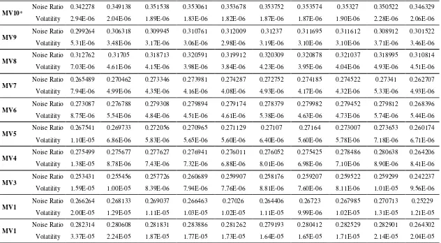
Table I reports noise proportion and return volatility computed according to the definition
above, by market capitalization and intraday interval. This noise proportion is shown I to be, at any
given day, the lowest at market open. Also, noises for small cap stocks, unlike volatilities, are lower
than those for large cap stocks, contrary to findings of Stoll (2000). Volatilities and noise
proportions of small-cap stocks exhibit in general a U-shaped pattern across a trading day, but noise
for large-cap stocks tend to go up from open to close. The intraday distribution of noise ratio for
small-caps is consistent with similar friction measures found in Hong Kong by Anh and Cheung
A measure of herding
We consider trading activity more in an dynamic sense by measuring order intensity not by
quantity, but by it sequences based on Patterson and Sharma (2006, PS). It captures intraday order
flows better than the popular LSV method, which is more suitable for longer time frame. In the
context of investor herding, we adopt a cost-based framework of trading concentration to see how
return volatility decomposition should be evaluated. The dynamic trading intensity allows us
capturing how ‘friction’ really arises from trades. As search cost goes up, so does noise. However,
search generates less noise at market open than at market close. Therefore, noise is lower when
specific search cost prevails, and noise gets higher when general friction rises.
To gauge the extent of trading concentration, we have adopted a dynamic measure specifically
for a high frequency trading environment. The common LSV measure computes the proportion of
market participants buying or selling within a given period and hence cannot capture dynamic order
flows. Its inference relies on conventional t-test, making it subject to distributional imperfections
especially with high frequency data. As a result, various measures have been proposed lately to
overcome its limitations. Radalj and McAleer (1993) noted that the main reason for the lack of
empirical evidence of herding may lie in the choice of data frequency, in the sense that too
infrequent data sampling would lead to intra-interval herding being missed (at monthly, weekly,
daily or even intra-daily intervals). For the purposes of our investigation we used the PS measure,
which we consider the most suitable, since it overcomes this problem of intraday data. Constructed
from intraday data, it has a major advantage of not assuming herding to vary with extreme market
conditions, and considering the market as a whole rather than a just the institutional investors.
PS statistic measures herding intensity in terms of the number of runs. The bootstrapped
runs test of PS uses run numbers of buy and sells orders3. As our data set contains identification of
buy or sell orders, we would not need Lee and Ready (1991) and Finucane (2002) to determine
directions of investors’ trading directions. If traders engage in systematic herding, the statistic
should take significantly negative values, since the actual number of runs will be lower than
expected. The standardized and adjusted type i runs for stock j on day t in PS is defined as
2 , 1 ) 1 ( ) 2 1 ( ) , ,
( = + − − i=
n
p np r
t j i
x i i i (4)
Where ri is the actual number of type i runs (up runs, down runs or zero runs), n is the total number of
3
trades executed on asset j on day t, ½ is a discontinuity adjustment parameter and p i is the
probability of finding a type of run i. Under asymptotic conditions, the statistic x(i,j,t) has a
normal distribution with zero mean and variance
2 2
2
) 1 ( 3 ) 1 ( ) , ,
(i j t = pi −pi − pi − pi
σ (5)
So the herding intensity statistic is expressed as
) , , (
) , , ( ) , , (
2 t j i
t j i x t j i H
σ
= (6)
which has an asymptotic distribution of N(0,1). Mood (1940) requires state variables to be
independent and i.i.d. as well as continuously distributed. As realized transaction price of stock is
discrete, H(i,j,t) would have a non-normal distribution and critical values for testing the
existence of herding would have to be constructed through bootstrapping the sample.
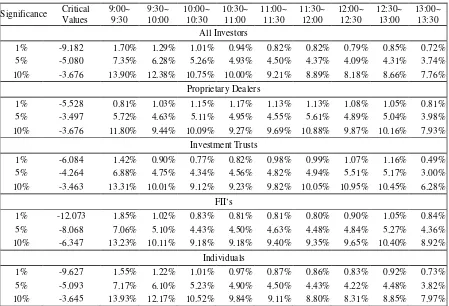
The distribution of significant herding percentage, as shown in Table II, suggests that intraday
trading concentration is heavier in the opening interval. At the 5% significance level, there are
7.35% of the trading days exhibit herding phenomenon in the first half hour of a day’s trading
session. The percentage falls as with time of day and goes down to only 3.74% for the final half
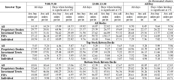
hour of trading. Table III gives the sizes of buy and sell orders, in lots of one thousand shares, for all
days where herding is significant at 1%. The average order size at market close is much larger than
in other periods. The ratios of average buy orders to average sell orders, for days when herding is
significant at 1%, is slightly higher than for the entire period. Among investor types, buy-sell ratios
are greater than 1 for all institutionals during days of herding. Looking further into the opening
intervals, we find that overall buy-sell ratios during significant herding days are actually lower than
the entire period. But for the closing interval, not only the ratios are generally higher than those in
the opening interval, but those in significant herding days are also higher than in the entire period.
This pattern coincides with intraday trading noise, which rises from open to close. If we look at
stocks in the top and bottom return deciles, the buy-sell ratios are, as expected, higher in the top
return decile. In the bottom return decile, buy-sell ratios are in general smaller than 1. Buy-sell
ratios in the closing intervals are uniformly higher, around 20%, than in the opening intervals. Even
for the bottom return decile, there appears to be a stronger, about 24% in magnitude, buying force
Market Width
Limit order book dispersion can describe the tightness of the book by examining how far apart
from each other (or from the midquote) the limit orders are placed in the book. It can also be considered
as the width of a market and it captures the execution price innovation expected by the limit order trader
when he sacrifices demand of immediacy and instead provides liquidity to the market. Foucault, Kadam,
and Kandel (2005) suggest that the limit order book dispersion is linked with the patience of limit order
traders and the pick-off risk they face. We adopt the following market width measure by modifying the
dispersion measure of Kang and Yeo (2008). The market width of stock i in a given day is defined as
+ =
= =
= =
5
1 5
1 5
1 5
1
2 1
j s j j
s j s j
j b j j
b j b j
i
w Dst w
w Dst w
MW (7)
where Dstbjis the price interval between the jth best buy order price and its next better order price, and
similarly Dstsj is that for the sell order price. The buy and sell price intervals, up to the fifth best limit
orders are weighted by wbj and
s j
w , the size of the corresponding buy or sell limit orders. For the
whole market, transaction prices are used to compute the first price interval, while for each type of
investors, average of buy and sell order price at each priority level is used instead. This dispersion, or
market width, measure is designed to show how clustered or dispersed the limit orders are in the book. It
measures how tightly the orders are placed to each other or how closely they are to the midquote. The
higher the dispersion is, the less tight the book is, and the lower amount of liquidity the limit order book
provides.
It is a well known fact in Taiwan that, due to funding liquidity, individual investors tend to hold
and trade stocks with lower prices, while institutional investors concentrate more on high price stocks.
Therefore, Dstbj and
s j
Dst in (7) are computed using the raw price distance divided by tick size of
the stock, so that only the relative price distance is used, allowing MWi to be comparable across stocks
and various types of investors.
Market Depth
Bloomfield, O’Hara, and Saar (2005) argue that informed traders would submit more limit
orders than market orders in an electronic market. McKenzie (2007) argues that in the emerging
markets especially the ability to forecast future price movements is related to the depth of those
book handles large volume of market orders. A deep limit order book can absorb a sudden surge in
the demand of liquidity without inducing much price deviation. Without the interference of the
specialist and before new limit orders can replenish the book, market buy (sell) orders will first be
executed against the limit sell (buy) orders at the best offer (bid) quote. If the volume of the market
order(s) is larger than the best offer (bid) size, the remainder of the unexecuted market orders will
be executed against the limit orders queuing at the next best offer (bid) quote. In other words, large
volume of market buy (sell) orders will walk up (down) the limit order book to get filled. The
further away the market orders walk up or down the book, the larger the difference between the
execution price and the mid-quote is, and therefore the more costly the trading process will be for
the market order traders. Motivated by the mechanism described above, we modify the market
depth measure of Kang and Yeo (2008), which can be thought of as an enhanced depth measure for
the limit order book.
i i K k i S k S k K k B k i B k i MQ TNS MQ P I P MQ I MD × − + −
= =1 =1
) (
) (
, (8)
where i=1,2,…,525. MQi is the midpoint of the nearest buy and sell quote prices, TNSi is the
total number of shares traded within the time interval of interest, PkB is the best bid price, PkS is
the best offer price and,
< > − > = = − = = = otherwise Q TNS and Q TNS if Q TNS Q TNS if Q I k j B j k j B j k j B j k j B j B j B k 0 ) ( 1 1 1 1 1 < > − > = = − = = = otherwise Q TNS and Q TNS if Q TNS Q TNS if Q I k j S j k j S j k j S j k j S j S j S k 0 ) ( 1 1 1 1 1
This study employs intra-day order book data from the Taiwan Stock Exchange starting from
March 1st, 2005 to December 31st, 2006, covering stocks of 525 firms over a period of 461 trading
days. Excluded from the complete pool of stocks listed on the exchange are those with irregularities
and unusual exchange sanctions. As the Taiwan Stock Exchange would only release limit book data
two years after an order or trade is realized, the data period the latest we could obtain. Each data
record includes date, exact time in hours, minutes and seconds, stock code, price and quantity of all
orders, filled or not, submitted during the data period. Individual stock returns, market
capitalizations, daily turnover and price-book ratios are obtained from the Taiwan Economic Journal
(TEJ) database.
Each daily session is then divided further into 9 intervals between 9:00 AM and 1:30 PM, with
30 minutes in each interval. As our data contains flags identifying each investor as either a
proprietary dealer, an investment trust, a FII or an individual, we are able to extend our analysis
according to investor types. Over the last ten years, percentages of trades in Taiwan stock market
accounted for by FII’s have apparently grown much faster than the other two types of local
institutionals. As a matter of fact, FII’S owns one third of the total market capitalization and account
for one quarter of daily volume as of end of 2009 in Taiwan. On average, about 15% of the daily
orders are submitted during the first half hour of a regular four and half hour trading session. In the
last half hour period, the percentages range between 9% and 19%. Trading in other periods is
usually slower than open and close.
To construct the herding intensity measures required for our study, we begin by sorting the
trades for each day (having excluded all those executed outside normal trading hours) by stock code
and count the numbers of up and down runs of order prices submitted within a given day, as well as
within each of the nine 30-minute intervals. We then compute herding statistic in the respective
periods according to PS (2006). The definition (6) usually makes computed herding measures take
on negative values. In computing PS herding measures, only the orders actually filled are included
in the computation to avoid reporting unrealistic herding phenomenon. The computed daily herding
measures in are larger in magnitudes than when they are computed intra-day, consistent with Dorn,
Huberman and Sengmueller (2008) which argue that herding measures should rise with length of
period. For all and each type of investors, we bootstrapped their 1%, 5% and 10% critical values.
Among all types of investors, FII’s exhibit the strongest herding behavior in the opening interval,
followed by individuals and investment trusts. Herding of proprietary dealers is quite different from
the other three types, peaking at mid-day sessions.
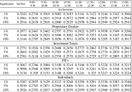
We report in Table IV the noise proportion in return volatility in the presence of trading
intend to identify possible factor driving trading noise. Does trading noise get heavier when market
is extremely active? According to the argument of Hu (2006) and Stoll (2000), a general transaction
cost should apply to everyone in the market, regardless of market capitalization of stocks or which
trading hour it is. Although noise is high on individual orders and low on institutional orders, it is
especially low at market open than in the rest of the day. For individuals, noise rises with
significance of herding as shown in Table IV, but not so for institutional investors. So trading noise
maybe just a specific transaction cost, as information cost, prominent to only certain investors in the
market.
In order to explore the effects of herding alone on noise in trading, we use the model below to
see its influences. We perform a panel regression with generalized least squares random effect based
on
t k t k t
k AH
N , =α+β , +ε , (9)
where N stands for noise as defined in (3), and H is defined according to (6). Also, t=1,…,461 (for
trading days) and k=1,…,525 (for stocks) . A greater in magnitude implies stronger noise is
produced by more intensive trading activity. Table V gives the result of this model, where a negative
estimate would indicates that trading activity brings in more trading noise, as herding measure
summarized in Table II in general takes on negative values. For the entire observations, the
magnitudes of coefficients in general peak at mid-day, with the closing interval having the weakest
coefficient. If we narrow the observations down to only those with significant herding at 10%, the
magnitudes of coefficients fall by 50%. When market opens, trading brings in the least amount of
noise. In another word, although noise does rise with herding, but when herding is very strong, its
influence on trading noise is actually smaller. When trading is not heavy, it affects noise more, but
not otherwise.
Table V reports the summary statistics of the market width measure, which shows why trading
could bring in more friction in the market. MW at each intraday interval, for the whole market or
various types of investors, is achieved by first subtracting the daily measure and then dividing by it,
which assures comparability across investor type. The market width measures are reported with a
layout with time-size blocks. As the computed value of measure is affected in practice by the arrival
rate of orders within a given time, figures in the table is modified to reflect the percentage each cell
in the block is above or below corresponding daily averages. MW increases in market capitalization,
as various friction measures mentioned in Stoll (2000). Also, it falls roughly from open to close,
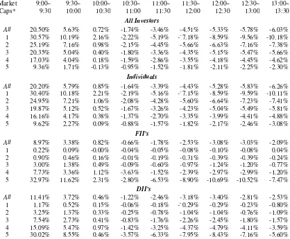
again consistent with Anh and Cheung (1999), but the difference between open and close decreases
more friction in the market. Taking investor type into consideration, we are able to see more
prominent northwest-southeast block polarization, with MW being polarized the most for
individuals and the least for FII’s. In fact, order width goes up with firm size on orders submitted by
FII’s and domestic institutional investors (DII’s), contrary to the direction for individuals. The block
distribution by investor type in Table VI suggests that, across time of day, order width benefits
trading. But in the category of individuals, it benefits more when trading stocks of the smaller firms,
while for institutional investors higher dispersion benefits trading stocks of larger firms. This kind
of clientele distribution of trading activity is not compatible with information-based explanation,
especially why order price dispersion is higher, at market open, when trading is extremely heavy.
However, if MW is just a form of economic rent imposed by limit order traders to reflect the
benefits each trader can enjoy through shorter search time.
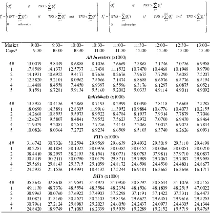
According to Table VII, the distribution of market depth, proxied by the depth of a limit order
book, is also compatible with our findings in previous tables. MD falls in general with both time of
day and firm size, uniformly across all types of investors. Order depth across firm size is compatible
with what frictions behave in Stoll (2000). The distribution across time of day is also consistent
with the findings of Anh and Cheung (1999) on intraday friction measures. Intraday trading activity
lowers order depth, and hence elevates market friction. Although stocks of larger firms possess
better depth, orders from individuals have on average more depth than those from institutional
investors. At market open, this edge is about 2.4 times, and increases to 3.9 times at market close.
Along the direction of firm size, individuals’ edge in order book depth at market open is 2.1 times
on small cap and 2.3 times on large cap, but is 3.7 times and 2.7 times respectively at market close.
So the results on market depth measure in Table VII implies that it is in the interest of FII’s and
DII’s to trade large cap stocks, especially at market close. For individuals, order book depth
indicated they should make the similar trading decision as the institutional investors to avoid higher
execution cost in trading small cap stocks at market open. However, the search cost advantage
dominates the execution cost. Apparently, for individuals finding a counterparty to complete an
intended trade is more important than walking up a few ticks on the limit order book and paying for
a slightly higher transacted price. After all, not being able to submit a market order in the Taiwan
market is itself a strong protection against shallow limit order book. Besides, there is also a 7%
price limit on either direction. Actual trading intensity may depend in part on the relative strength of
search and execution costs.
Based on a framework of time-size block, we show why intraday trading could actually result
more friction in a market. The relation is, however, on the level of broad categories. To determine
point estimations. We use the following model to find out how order width affects actual time it
takes to fill a buy order. A fixed effect panel regression is performed on
t k t k t
k MW
N , =
α
+γ
1 , +ε
, (10)where t=1,…,461 and k=1,…,525. Results are estimated using a panel GLS with AR(1)4
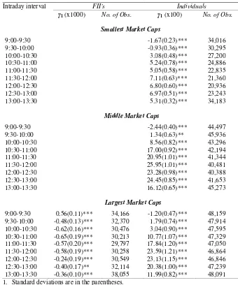
adjustments on residuals and reported in Table VIII, which suggests that order width affects market
friction in different ways across investor type and time of day. Similar to the previous models, the
model for domestic institutional does not pass the validation test again and only results for the
largest market capitalization are available for FII’s. For FII’s dispersion suppresses trading noise
significantly except for the first intraday interval. For the individuals, however, dispersion elevates
trading noise except for the first intraday interval regardless of market capitalizations. The exact
mirror type pattern that distinguish FII’s from individuals supports notion that heavy trading of
individuals at market open induces noise. For FII’s, aggressive order price pattern, or lower
dispersion, just produces lower trading noises at market open. In other intraday intervals, only more
aggressive order price pattern would produce greater trading noise, confirming the findings of Table
VI.
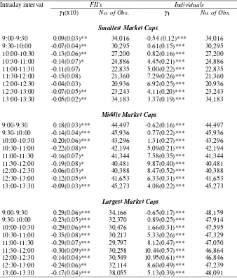
Table IX gives results showing how market depth affects trading noise. The following
model is considered for this purpose,
t k t k t
k MD
N , =
α
+γ
1 , +ε
, (11)where t=1,…,461 and k=1,…,525. Results are estimated using a panel GLS with AR(1) adjustments
on residuals. Table IX shows a similar pattern to that in Table VIII. Market depth of orders from
institutional investors, which is lower than the depth in individuals’ orders, contributes to trading
noise positively at market open. However, for the rest of the day, market depth of institutionals’
orders tends to suppress trading noise. The relation between trading noise and market depth is the
opposite of that at market open. For the institutional investors, market depth affects noise only
weakly on small cap stocks. Results from Tables VIII and IX validate the pattern of noise across a
day, as reported in Table IV. When the market is very active, in width or depth, trading noise of
investors actually benefit from heavy trading. This is especially true for individual investors at
market open, when poor width and depth actually hurts the institutional investors in bearing higher
trading noise.
IV. Conclusion
This study examines intra-day order book data to study whether trading activity incites or
suppresses certain market friction, particularly when trading is heavy. We adopt a measure of
trading concentration specifically ideal for high frequency data. The measure is not only constructed
on a daily level, but also within intra-day time intervals. Trading concentration is found to bring in
noise or friction to the market. As we find trading brings friction, our findings provide support to
the new financial transactions tax proposed by the European Union, which has invited lots of
criticism.
We have also introduced measures on width and depth of a limit order book to explain why
market friction reacts to trading activity as we find it. We find strong evidences against the idea of
trading noise being a general transaction cost, or a general friction in market trading. Specifically,
trading noise behaves, and reacts to market width and depth, differently across investor type, market
capitalization and time of day. Trading noise is just a specific transaction cost, as information cost,
prominent at certain aspect in the market.
Although this noise is high on individual orders and low on institutional orders, its behavior at
market open is entirely different from the rest of the day. Noises for small cap stocks, unlike
volatilities, are lower than those for large cap stocks. Intraday trading activity suppresses width, as
well as depth, of orders submitted, therefore creates more noise in the market. At market open,
behaviors of noise from institutional and individual orders are opposite to each other, but they
switch positions in the rest of the day. Noise from high-cap stocks is actually more responsive than
that from low-cap ones across investors. So trading noise is a specific transactions cost, prominent
to only certain investors, at certain time and for certain stocks in the market, rather than a general
market friction as argued in Stoll (2000). This transactions cost is inversely related to order width
and depth, which depends on investor, trading hour of day and market capitalization of stocks.
Although we have presented valid arguments regarding the central issue of this study, there are
areas yet to be worked on. We have to investigate further behavior of trading noise and its
interaction with investors. Other analysis, such as trading motives of investors, evidence on
sequence or development of trading concentration and the dynamics of trading noise need to be
References
1. Admati, A. R., (1991), “The Informational Role of Prices,” Journal of Monetary Economics
28,347-361.
2. Ahn, H. and Cheung, Y.. (1999), “The intraday patterns of the spread and depth in a market
without market makers: The Stock Exchange of Hong Kong,” Pacific-Basin Finance Journal 7,
539-556.
3. Amihud, Y. and Mendelson, H.. (1987), “Trading mechanism and stock returns: An empirical
investigation,” Journal of Finance 42, 533-553.
4. Avery, C. and Zemsky, P.. (1998), “Multidimensional uncertainty and herd behavior in
financial markets,” American Economic Review 88, no. 4, 724-748.
5. Banerjee, A.. (1992), “A Simple Model of Herd Behavior,” Quarterly Journal of Economics
107, 797-817.
6. Bikhchandani, S.; Hirshleifer, D.; Welch, I.. (1992), “A Theory of Fads, Fashion, Custom, and
Cultural Change as Informational Cascades,” Journal of Political Economy 100, 992-1026.
7. Chang, E. C.; Cheng, J. W.; Khoran, A., (2000), “An examination of herd behavior in equity
markets: An international perspective,” Journal of Banking and Finance 24, no. 10,
1651-1699.
8. Chakraborty, A. and Yilmaz, B., (2004), "Manipulation in market order models," Journal of
Financial Markets 7(2), 187-206.
9. Cont, R. and Bouchaud, J. P.. (2000), “Herd Behavior and Aggregate Fluctuations in Financial
Markets,” Macroeconomic Dynamics 4, 170-196.
10. De Long, J. B., A. Shleifer, L. H. Summers, and R. J. Waldmann, (1990), “Positive Feedback
Investment Strategies and Destabilizing Rational Speculation,” Journal of Finance 45(2),
374-397.
11. Diamond, D. W., and Verrecchia, R. E., (1981), “Information Aggregation in a Noisy Rational
Expectations Economy,” Journal of Financial Economics 9, 221-235.
12. Dorn, D.; G. Huberman; P. Sengmueller. 2008. “Correlated Trading and Returns.” Journalof
Finance 58, no. 2: 885-920.
13. Easley, D., Kiefer, N. M., and O’Hara, M., (1997), “One Day in the Life of a Very Common
Stock,” Review of Financial Studies 10, 805-835.
14. Easley, D., and O’Hara, M., (1992), “Time and the Process of Security Price Adjustment,”
Journal of Finance 47, 577-605.
15. Finucane, T. J.. (2002), “A Direct Test of Methods for Inferring Trade Direction from Intra-day
Data,” Journal of Financial and Quantitative Analysis 35, 553-557.
16. Foucault, T., Kadam, O., and Kandel, E., (2005), “Limit Order Book as a Market for
Liquidity, ” Review of Financial Studies 18, 1171-1218.
17. Glosten, L. R. and Milgrom, P. R., (1985), “Bid, ask and transaction prices in a specialist
market with heterogeneously informed traders,” Journal of Financial Economics, Vol. 14(1),
Markets,” American Economic Review 70(3), 393-408.
19. Hu, S.. (2006), “A Simple Estimate of Noise and Its Determinant in a Call Auction Market,”
International Review of Financial Analysis 15, 348-362.
20. Jarrow, R.. (1992), “Market manipulations, bubbles, corners and short squeezes,” Journal of
Financial and Quantitative Analysis 27, 311-336.
21. Kang, W., and Yeo, W., (2008), “Liquidity beyond the Best Quote: A Study of the NYSE Limit
Order Book,” Working Paper, National University of Singapore.
22. Kyle, A. S., (1985), “Continuous Auctions and Insider Trading,” Econometrica 53, 1315-1335.
23. Lakonishok, J.; Shleifer, A.; Vishny, R. W., (1992), “The Impact of Institutional Trading on
Stock Prices,” Journal of Financial Economics 32, 23-43.
24. Lee, C. M. C., and Ready, M. J., (1991), “Inferring Trade form Intraday Data,” Journal of
Finance 46, 733-746.
25. Lin, J., Sanger, G. C., and Booth, G. G., (1995). “Trade size and components of the bid-ask spread,” Review of Financial Studies 8, 1153−1183.
26. Lin, W. T., Tsai, S. C., and Sun, D. S., (2011), “Search Costs and Investor Trading Activity:
Evidences from limit order book,” Forthcoming, Emerging Markets Finance and Trade.
27. McKenzie, M.D. (2007). Technical Trading Rules in Emerging Markets and the 1997 Asian
Currency Crises, Emerging Markets Finance and Trade, 43, 46-73.
28. Mood, A., (1940), “The distribution theory of runs,” Annals of Mathematical Statistics 11,
367-392.
29. Nofsinger, J. R., and Sias, R.W.. (1999), “Herding and Feedback Trading by Institutional and
Individual Investors,” Journal of Finance 54, 2263-2295.
30. Patterson, D., and Sharma, V.. (2006), “Do Traders Follow Each Other at the NYSE?” Working
Paper, University of Michigan-Dearborn.
31. Radalj, M., and McAleer, M.. (1993). “Herding, information cascades and volatility spillovers
in futures markets,” Working Paper, University of Western Australia, Perth, Australia.
32. Stoll, H.R.. “Friction,” Journal of Finance 55 (2000), 1479-1514.
33. Stoll, H. R., and R. E. Whaley, (1990), “Stock market structure and volatility,” Review of
Financial Studies, Vol. 3, pp.37−71.
34. Wermers, R.. “Mutual Fund Herding and the Impact on Stock Prices,” Journal of Finance, 54
Table I Noise as Proportion of Stock Returns by Market Capitalization and Intraday Interval Averaged across 525 firms and over 461 days
9:00~9:30 9:30~10:00 10:00~10:30 10:30~11:00 11:00~11:30 11:30~12:00 12:00~12:30 12:30~13:00 13:00~13:30 all day
MV10* Noise Ratio 0.342278 0.349138 0.351538 0.353061 0.353678 0.353752 0.353574 0.35327 0.350522 0.346329
Volatility 2.94E-06 2.04E-06 1.89E-06 1.83E-06 1.82E-06 1.87E-06 1.87E-06 1.90E-06 2.28E-06 2.06E-06
MV9
Noise Ratio 0.299264 0.306318 0.309945 0.310761 0.312009 0.31237 0.311695 0.311612 0.308912 0.301522 Volatility 5.31E-06 3.48E-06 3.17E-06 3.06E-06 2.98E-06 3.19E-06 3.10E-06 3.10E-06 3.71E-06 3.46E-06
MV8
Noise Ratio 0.312762 0.31705 0.318713 0.320591 0.319912 0.320309 0.320878 0.321037 0.318995 0.310814 Volatility 7.03E-06 4.61E-06 4.15E-06 3.98E-06 3.84E-06 4.23E-06 3.95E-06 4.04E-06 4.93E-06 4.51E-06
MV7 Noise Ratio 0.265489 0.270462 0.273346 0.273981 0.274287 0.272752 0.274185 0.274522 0.27341 0.262707
Volatility 7.94E-06 4.99E-06 4.35E-06 4.16E-06 4.08E-06 4.93E-06 4.17E-06 4.32E-06 5.33E-06 4.93E-06
MV6 Noise Ratio 0.273087 0.276788 0.279308 0.279894 0.279174 0.278379 0.279982 0.279452 0.279812 0.268396
Volatility 8.75E-06 5.54E-06 4.84E-06 4.51E-06 4.61E-06 5.38E-06 4.63E-06 4.73E-06 5.74E-06 5.44E-06
MV5 Noise Ratio 0.267541 0.269733 0.272056 0.270965 0.271129 0.27107 0.27164 0.273007 0.273653 0.260174
Volatility 1.10E-05 6.86E-06 5.83E-06 5.65E-06 5.60E-06 6.40E-06 5.60E-06 5.78E-06 7.18E-06 6.71E-06
MV4 Noise Ratio 0.275499 0.275677 0.277627 0.276941 0.276011 0.276052 0.275425 0.278486 0.280638 0.264206
Volatility 1.38E-05 8.78E-06 7.43E-06 7.32E-06 6.88E-06 8.01E-06 6.98E-06 7.10E-06 8.90E-06 8.41E-06
MV3 Noise Ratio 0.253431 0.255456 0.257726 0.260689 0.259907 0.258176 0.259207 0.259522 0.259299 0.242237
Volatility 1.59E-05 1.00E-05 8.39E-06 7.94E-06 7.76E-06 8.81E-06 7.60E-06 8.11E-06 1.01E-05 9.56E-06
MV1 Noise Ratio 0.266264 0.268133 0.269037 0.266463 0.27026 0.264406 0.26723 0.267985 0.270713 0.25229
Volatility 2.00E-05 1.29E-05 1.11E-05 1.03E-05 1.02E-05 1.11E-05 9.99E-06 1.02E-05 1.31E-05 1.21E-05
MV1 Noise Ratio 0.282314 0.280608 0.281831 0.283886 0.281262 0.279193 0.280412 0.282529 0.282901 0.264302
[image:19.792.72.704.135.483.2]Table II Bootstrapped Intra-day Critical Values and Herding Significance Percentages by Intraday Intervals and Investor Type, Averaged across 525 firms and over 495 days
Significance Critical Values
9:00~ 9:30
9:30~ 10:00
10:00~ 10:30
10:30~ 11:00
11:00~ 11:30
11:30~ 12:00
12:00~ 12:30
12:30~ 13:00
13:00~ 13:30 All Investors
1% -9.182 1.70% 1.29% 1.01% 0.94% 0.82% 0.82% 0.79% 0.85% 0.72% 5% -5.080 7.35% 6.28% 5.26% 4.93% 4.50% 4.37% 4.09% 4.31% 3.74% 10% -3.676 13.90% 12.38% 10.75% 10.00% 9.21% 8.89% 8.18% 8.66% 7.76%
Proprietary Dealers
1% -5.528 0.81% 1.03% 1.15% 1.17% 1.13% 1.13% 1.08% 1.05% 0.81% 5% -3.497 5.72% 4.63% 5.11% 4.95% 4.55% 5.61% 4.89% 5.04% 3.98% 10% -3.676 11.80% 9.44% 10.09% 9.27% 9.69% 10.88% 9.87% 10.16% 7.93%
Investment Trusts
1% -6.084 1.42% 0.90% 0.77% 0.82% 0.98% 0.99% 1.07% 1.16% 0.49% 5% -4.264 6.88% 4.75% 4.34% 4.56% 4.82% 4.94% 5.51% 5.17% 3.00% 10% -3.463 13.31% 10.01% 9.12% 9.23% 9.82% 10.05% 10.95% 10.45% 6.28%
FII’s
1% -12.073 1.85% 1.02% 0.83% 0.81% 0.81% 0.80% 0.90% 1.05% 0.84% 5% -8.068 7.06% 5.10% 4.43% 4.50% 4.63% 4.48% 4.84% 5.27% 4.36% 10% -6.347 13.23% 10.11% 9.18% 9.18% 9.40% 9.35% 9.65% 10.40% 8.92%
Individuals
Table III Daily and Intra-day Buy and Sell Orders, All Days and When Herding Is Significant at 1%
By Investor Type
Investor Type
9:00~9:30 13:00~13:30 All Day
All days Days when herding is significant at 1%
All days Days when herding is significant at 1%
All days Days when herding is significant at 1% Ave. buy
orders per lot
Ave. sell orders per lot
Ave. buy orders per lot
Ave. sell orders per lot
Ave. buy orders per lot
Ave. sell orders per lot
Ave. buy orders per lot
Ave. sell orders per lot
Ave. buy orders per lot
Ave. sell orders per
lot
Ave. buy orders per
lot
Ave. sell orders per
lot
All Stocks
All 14.19 14.24 15.09 18.33 19.92 18.07 22.82 18.53 8.50 8.45 9.64 9.56
Proprietary Dealers 29.77 24.81 68.96 15.11 23.37 25.39 26.57 19.69 21.66 22.17 26.22 8.61
Investment Trusts 41.53 31.41 56.62 29.49 31.58 27.62 66.09 53.32 28.68 25.34 13.77 12.88
FII’s 27.12 26.18 43.95 25.22 69.19 59.72 130.17 26.60 17.10 17.34 14.05 12.39
Individual 10.54 11.12 10.05 22.82 9.76 10.18 9.66 17.31 7.29 7.36 7.02 7.67
Top Stock Return Decile
All 5.43 5.24 6.46 5.87 5.67 5.29 7.15 5.65 5.44 5.28 5.99 5.96
Proprietary Dealers 17.95 15.20 6.36 12.28 11.91 12.60 9.25 12.80 14.96 14.39 6.49 5.33
Investment Trusts 25.99 17.91 25.48 18.95 22.56 17.95 14.28 5.22 19.33 16.13 11.66 11.08
FII’s 7.93 6.76 4.73 3.95 13.30 12.61 5.88 4.24 7.52 7.06 4.28 3.90
Individual 5.02 4.95 5.47 5.32 5.00 4.83 3.00 3.07 5.02 4.94 5.18 5.33
Bottom Stock Return Decile
All 10.81 10.64 15.53 13.06 12.39 12.39 18.76 12.67 10.53 10.85 10.17 12.83
Proprietary Dealers 32.68 31.13 34.55 20.14 26.12 29.81 56.59 37.77 25.82 28.30 31.04 12.15
Investment Trusts 58.67 46.06 180.25 24.81 41.04 31.32 45.81 56.36 39.80 34.26 14.58 13.49
FII’s 18.88 18.87 19.95 6.95 45.79 46.07 39.87 42.69 20.61 20.84 18.02 10.53
Individual 10.22 9.98 12.58 12.53 9.92 10.18 9.35 10.77 9.64 9.91 8.64 10.71
Table IV Noise as Proportion of Stock Returns by Herding Significance Averaged across 525 firms and over 495 days
Significance All Day 9:00~ 9:30
9:30~ 10:00
10:00~ 10:30
10:30~ 11:00
11:00~ 11:30
11:30~ 12:00
12:00~ 12:30
12:30~ 13:00
13:00~ 13:30 All Investors
1% 0.3242 0.2718 0.3010 0.3082 0.3183 0.3161 0.3122 0.3144 0.3162 0.3066
5% 0.2981 0.2651 0.2833 0.2918 0.2972 0.2995 0.2984 0.2970 0.2957 0.2944
10% 0.2916 0.2678 0.2816 0.2880 0.2929 0.2958 0.2944 0.2949 0.2924 0.2943
Proprietary Dealers
1% 0.2977 0.2467 0.2462 0.2557 0.2791 0.2822 0.2973 0.3038 0.3349 0.3206
5% 0.3144 0.2624 0.2822 0.3006 0.3082 0.2957 0.3253 0.3101 0.3165 0.3036
10% 0.3144 0.2705 0.2849 0.3056 0.3031 0.3076 0.3304 0.3205 0.3187 0.3017
Investment Trusts
1% 0.2751 0.1924 0.2358 0.2688 0.2456 0.2773 0.2862 0.2736 0.2778 0.2861
5% 0.2602 0.2042 0.2429 0.2583 0.2573 0.2675 0.2758 0.2774 0.2870 0.2917
10% 0.2581 0.2118 0.2410 0.2554 0.2570 0.2673 0.2729 0.2737 0.2805 0.2873
FII’s
1% 0.3067 0.2766 0.3084 0.3100 0.3214 0.3166 0.3217 0.3224 0.3218 0.3215
5% 0.3098 0.2968 0.3099 0.3158 0.3205 0.321 0.3241 0.3211 0.3198 0.3192
10% 0.3136 0.305 0.3153 0.3188 0.3200 0.3241 0.325 0.3217 0.3224 0.3224
Individuals
1% 0.3387 0.2855 0.3129 0.3212 0.3268 0.3294 0.3291 0.3336 0.3383 0.3346
5% 0.3030 0.2703 0.2871 0.2964 0.3006 0.3011 0.3016 0.3044 0.3037 0.3050
[image:22.612.88.527.116.421.2]Table V Effects of Herding on Noise in Panel Regression Intraday Intervals
In order to explore the effects of trading concentration alone on trading noise, we use the model below to see what could have influenced noise. We performed a panel regression with generalized least squares random effect based on
t k t k t
k H
N , =α+β , +ε ,
where N stands for noise as defined in (3), and H is defined according to (6). Also, t=1,…,461 (for trading days) and k=1,…,525 (for stocks) . A greater in magnitude implies stronger noise is produced by more intensive trading activity.
Intraday interval (x100) No of obs.
All days
9:00-9:30 -1.32(0.0128)*** 222,711 9:30-10:00 -1.21(0.0140)*** 217,529 10:00-10:30 -1.34(0.0153)*** 213,436 10:30-11:00 -1.45(0.0161)*** 209,637 11:00-11:30 -1.53(0.0168)*** 206,076 11:30-12:00 -1.59(0.0170)*** 202,803 12:00-12:30 -1.56(0.0173)*** 202,750 12:30-13:00 -1.30(0.0166)*** 208,049 13:00-13:30 -0.98(0.0161)*** 222,387
Days when herding is significant at 10%
9:00-9:30 -0.25(0.0128)*** 22,298 9:30-10:00 -0.45(0.0140)*** 21,815 10:00-10:30 -0.62(0.0153)*** 21,402 10:30-11:00 -0.79(0.0161)*** 20,944 11:00-11:30 -0.83(0.0168)*** 20,650 11:30-12:00 -0.85(0.0170)*** 20,416 12:00-12:30 -0.86(0.0173)*** 20,464 12:30-13:00 -0.74(0.0166)*** 20,959 13:00-13:30 -0.54(0.0161)*** 22,497 1.Standard deviations are in the parentheses.
Table VI Summary Statistics of Intraday Market Width Relative to Daily Average 525 firms and over 461 days
The dispersion measure of stock i in a given day is defined as
+ × = = = = = n j s ij n j S ij S ij n j B ij n j B ij B ij i i w D w w D w Tick MW 1 1 1 1 2 1
where i=1,2,…,525 and Ticki is the tick size of the respective stock. ( i,j1 ij) B
ij Bid Bid
D = − − , which is the price interval between the jth best bid order price and the next better quote, whereas DijS =(Offeri,j−1−Offerij), which is the price interval between the jth best offer order price and the next better quote, with wij being the size of the corresponding bid or offer order. For the whole market, transaction prices are used to compute the first price interval, while for each type of investors, average of buy and sell order price at each priority level is used instead. As the computed value of measure is affected in practice by the arrival rate of orders within a given time, figures in the table is modified to reflect the percentage each cell in the block is above or below corresponding daily averages.
Market Caps* 9:00~ 9:30 9:30~ 10:00 10:00~ 10:30 10:30~ 11:00 11:00~ 11:30 11:30~ 12:00 12:00~ 12:30 12:30~ 13:00 13:00~ 13:30 All Investors
All 20.50% 5.63% 0.72% -1.74% -3.46% -4.51% -5.33% -5.78% -6.03% 1 30.57% 10.19% 2.16% -2.22% -5.19% -`7.18% -8.59% -9.56% -10.18% 2 25.19% 7.16% 0.98% -2.15% -4.45% -5.66% -6.63% -7.16% -7.38% 3 20.35% 5.04% 0.40% -1.80% -3.36% -4.35% -5.15% -5.47% -5.66% 4 17.03% 4.04% 0.18% -1.59% -2.86% -3.55% -4.18% -4.45% -4.62% 5 9.36% 1.71% -0.13% -0.95% -1.52% -1.81% -2.11% -2.25% -2.30%
Individuals
All 20.20% 5.79% 0.85% -1.64% -3.39% -4.43% -5.28% -5.83% -6.26% 1 30.40% 10.18% 2.21% -2.19% -5.16% -`7.15% -8.59% -9.59% -10.11% 2 24.95% 7.21% 1.06% -2.08% -4.28% -5.60% -6.64% -7.23% -7.41% 3 19.87% 5.12% 0.52% -1.67% -3.26% -4.23% -5.04% -5.49% -5.81% 4 16.16% 4.17% 0.38% -1.37% -2.70% -3.35% -3.99% -4.41% -4.88% 5 9.62% 2.27% 0.09% -0.88% -1.57% -1.82% -2.17% -2.46% -3.08%
FII’s
All 8.97% 3.38% 0.82% -0.66% -1.78% -2.53% -3.08% -3.03% -2.09% 1 0.22% 0.09% -0.00% -0.04% -0.05% -0.08% -0.10% -0.08% 0.04% 2 0.90% 0.46% 0.16% -0.01% -0.19% -0.31% -0.39% -0.39% -0.24% 3 3.00% 1.38% 0.49% -0.09% -0.60% -0.97% -1.24% -1.20% -0.77% 4 7.73% 3.36% 1.12% -3.63% -1.52% -2.39% -2.97% -2.99% -1.20% 5 32.97% 11.62% 2.31% -2.80% -6.53% -8.90% -10.69% -10.52% -7.47%
DII’s
[image:24.612.95.513.324.669.2]Table VII Summary Statistics of Intraday Market Depth Across 525 firms over 461 trading days
i i K k i S k S k K k B k i B k i MQ TNS MQ P I P MQ I MD × − + −
= =1 =1
) (
) (
,
where i=1,2,…,525. MQi is the midpoint of the nearest buy and sell quote prices, TNSi is the total number of shares traded within the time interval of interest, PkB is the best bid price, PkS is the best offer price and,
< > − > = = − = = = otherwise Q TNS and Q TNS if Q TNS Q TNS if Q I k j B j k j B j k j B j k j B j B j B k 0 ) ( 1 1 1 1 1 < > − > = = − = = = otherwise Q TNS and Q TNS if Q TNS Q TNS if Q I k j S j k j S j k j S j k j S j S j S k 0 ) ( 1 1 1 1 1 Market Caps* 9:00~ 9:30 9:30~ 10:00 10:00~ 10:30 10:30~ 11:00 11:00~ 11:30 11:30~ 12:00 12:00~ 12:30 12:30~ 13:00 13:00~ 13:30 All Investors (x1000)
All 13.0079 9.8449 8.6888 8.1036 7.6669 7.3865 7.1746 7.0736 6.9958 1 17.8589 14.1373 12.5737 11.7438 11.1532 10.7470 10.4468 10.1948 9.9790 2 14.1931 10.6952 9.4177 8.7636 8.2676 7.9675 7.7290 7.6085 7.5207 3 12.3820 9.2101 8.0962 7.5566 7.1474 6.8688 6.6576 6.5776 6.5194 4 11.4488 8.4558 7.4450 6.9397 6.5596 6.3176 6.1297 6.0875 6.0521 5 9.1591 6.7281 5.9134 5.5160 5.2082 5.0333 4.9114 4.9011 4.9092
Individuals (x1000)
All 13.3955 10.4136 9.2868 8.7193 8.2999 8.0390 7.8118 7.6603 7.5285 1 18.0690 14.3891 12.8305 11.9916 11.3952 10.9884 10.6776 10.4073 10.2155 2 14.2668 10.8553 9.5973 8.9522 8.4784 8.1937 7.9314 7.7879 7.7046 3 12.6287 9.5807 8.4841 7.9552 7.5623 7.2972 7.0700 6.9430 6.8464 4 11.9329 9.2087 8.2513 7.7756 7.4143 7.2065 7.0072 6.9023 6.7844 5 10.0826 8.0364 7.2727 6.9234 6.6509 6.5103 6.3740 6.2626 6.0931
FII’s (x1000)
All 31.6742 30.7326 30.2594 29.9569 29.6639 29.4932 29.3019 29.3110 29.4198 1 38.2287 38.1884 38.1322 38.0976 38.0382 38.0152 38.0066 38.0051 38.0210 2 38.4410 38.2997 38.2193 38.1541 38.0731 38.0783 37.9811 37.9710 38.0837 3 30.5419 30.2111 30.0790 30.0179 29.8711 29.7989 29.7067 29.7387 29.9595 4 25.5691 25.8143 25.3715 25.1059 24.8172 24.6598 24.4530 24.4801 24.8677 5 24.5935 21.1536 19.4991 18.4132 17.5244 16.9181 16.3665 16.3646 16.1717
DII’s (x1000)
Table VIII Effects of Market Width on Noise Foreign Institutional and IndividualInvestors, by Market Caps
To explore the effects of search motive on trading noise on an intraday level, we use the model below to see what could have influenced noise. We performed a panel regression with
generalized least squares random effect based on
t k t k t k MW
N, =α+γ1 , +ε , with +
× = = = = = n j s ij n j S ij S ij n j B ij n j B ij B ij i i w D w w D w Tick MW 1 1 1 1 2 1
and t=1,…,461 and k=1,…,525. MWk,tfollows the same definition as in (7). Results are estimated using a panel GLS with AR(1) adjustments on residuals.
Intraday interval FII’s Individuals
1 (x1000) No. of Obs. 1 (x100) No. of Obs.
Smallest Market Caps
9:00-9:30 -1.67(0.23)*** 34,016
9:30-10:00 -0.93(0.36)*** 30,295
10:00-10:30 3.08(0.48)*** 27,200
10:30-11:00 5.24(0.78)*** 24,886
11:00-11:30 5.05(0.58)*** 22,835
11:30-12:00 7.11(0.63)*** 21,360
12:00-12:30 6.80(0.60)*** 20,936
12:30-13:00 6.97(0.51)*** 23,243
13:00-13:30 5.31(0.32)*** 34,183
Middle Market Caps
9:00-9:30 -2.44(0.40)*** 44,497
9:30-10:00 1.34(0.63)** 45,936
10:00-10:30 8.56(0.82)*** 43,296
10:30-11:00 17.00(0.92)*** 42,194
11:00-11:30 20.95(1.01)*** 41,344
11:30-12:00 25.95(1.01)*** 40,481
12:00-12:30 23.28(0.98)*** 40,388
12:30-13:00 24.45(0.85)*** 41,653
13:00-13:30 16.12(0.65)*** 45,273
Largest Market Caps
9:00-9:30 0.56(0.11)*** 34,166 -1.20(0.47)*** 48,159 9:30-10:00 -0.48(0.13)*** 32,370 1.79(0.74)*** 47,914 10:00-10:30 -0.62(0.16)*** 30,476 3.04(0.90)*** 47,595 10:30-11:00 -0.65(0.19)*** 30,213 10.77(1.07)*** 47,329 11:00-11:30 -0.57(0.20)*** 29,797 17.84(1.20)*** 47,050 11:30-12:00 -0.58(0.19)*** 30,258 23.59(1.21)*** 46,864 12:00-12:30 -0.24(0.19)*** 30,549 23.13(1.15)*** 46,846 12:30-13:00 -0.40(0.17)** 32,114 20.38(1.00)*** 47,239 13:00-13:30 -0.36(0.10)*** 38,055 11.99(0.82)*** 48,091 1. Standard deviations are in the parentheses.
Table IX Effects of Market Depth on Noise Foreign Institutional and IndividualInvestors, by Market Caps
To explore the effects of search motive on trading noise on an intraday level, we use the model below to see what could have influenced noise. We performed a panel regression with
generalized least squares random effect based on
t k t k t k MD
N, =α+γ1 , +ε, with
k k I i k S i S i I i B i k B i k MQ TNS MQ P I P MQ I MD × − + −
= =1 =1
) (
) (
and t=1,…,461 and k=1,…,525. Results are estimated using a panel GLS with AR(1) adjustments on residuals.
Intraday interval FII’s Individuals
1(x10) No. of Obs. 1 No. of Obs.
Smallest Market Caps
9:00-9:30 0.09(0.03)** 34,016 -0.54 (0.12)*** 34,016 9:30-10:00 -0.07(0.04)** 30,295 0.61(0.15)*** 30,295 10:00-10:30 -0.13(0.06)** 27,200 0.82(0.16)*** 27,200 10:30-11:00 -0.14(0.07)* 24,886 4.45(0.21)*** 24,886 11:00-11:30 -0.11(0.07) 22,835 5.00(0.22)*** 22,835 11:30-12:00 -0.15(0.08) 21,360 7.29(0.26)*** 21,360 12:00-12:30 -0.04(0.03) 20,936 6.92(0.25)*** 20,936 12:30-13:00 -0.07(0.05)** 23,243 4.11(0.20)*** 23,243 13:00-13:30 -0.05(0.02)** 34,183 3.37(0.19)*** 34,183
Middle Market Caps
9:00-9:30 0.18(0.03)*** 44,497 -0.62(0.16)*** 44,497 9:30-10:00 -0.14(0.04)*** 45,936 0.77(0.22)*** 45,936 10:00-10:30 -0.20(0.06)*** 43,296 1.31(0.27)*** 43,296 10:30-11:00 -0.22(0.08)** 42,194 5.09(0.21)*** 42,194 11:00-11:30 -0.16(0.07)* 41,344 7.58(0.35)*** 41,344 11:30-12:00 -0.19(0.08)* 40,481 9.87(0.40)*** 40,481 12:00-12:30 -0.06(0.03)* 40,388 8.47(0.52)*** 40,388 12:30-13:00 -0.12(0.05)** 41,653 6.33(0.31)*** 41,653 13:00-13:30 -0.09(0.03)*** 45,273 4.08(0.22)*** 45,273
Largest Market Caps
9:00-9:30 0.29(0.06)*** 34,166 -0.65(0.17)*** 48,159 9:30-10:00 -0.23(0.05)*** 32,370 0.89(0.25)*** 47,914 10:00-10:30 -0.29(0.06)*** 30,476 1.66(0.31)*** 47,595 10:30-11:00 -0.35(0.08)*** 30,213 5.33(0.26)*** 47,329 11:00-11:30 -0.29(0.07)*** 29,797 8.12(0.47)*** 47,050 11:30-12:00 -0.30(0.09)*** 30,258 10.44(0.57)*** 46,864 12:00-12:30 -0.14(0.04)*** 30,549 10.95(0.61)*** 46,846 12:30-13:00 -0.24(0.06)** 32,114 8.60(0.49)*** 47,239 13:00-13:30 -0.17(0.04)*** 38,055 5.13(0.39)*** 48,091 1. Standard deviations are in the parentheses.