Vanilla Option Pricing on Stochastic Volatility market models

Munich Personal RePEc Archive

Vanilla Option Pricing on Stochastic

Volatility market models

Dell’Era, Mario

4 October 2010

Online at

https://mpra.ub.uni-muenchen.de/25645/

October 4, 2010

Vanilla Option Pricing on Stochastic Volatility market models

Mario Dell’Era

University Pisa, Mathematics and Statistics Department e-mail: m.dellera@ec.unipi.it

Abstract

1

Introduction

The Black-Scholes model rests upon a number of assumptions that are, to some extent, strategic. Among these there are continuity of stock-price process (it does not jump), the ability to hedge continuously without transaction costs, independent Gaussian returns, and constant volatility. We are going to focus here on relaxing the last assumption by allowing volatility to vary ran-domly, for the following reason, a well-known discrepancy between the Black-Scholes predicted European option prices and market-traded options prices, thesmile curve, can be accounted for by stochastic volatility models. Modeling volatility as a stochastic process is motivated a priori by empirical studies of stock-price returns in which estimated volatility is observed to exhibit random characteristics. Additionally, the effects of transaction costs show up under many models, as uncertainty in the volatility; fat-tailed returns distributions can be simulated by stochastic volatility. The assumption of constant volatility is not reasonable, since we require different values for the volatility parameter for different strikes and different expiries to match market prices. The volatility parameter that is required in the Black-Scholes formula to repro-duce market prices is called the implied volatility. This is a critical internal inconsistency, since the implied volatility of the underlying should not be dependent on the specifications of the contract. Thus to obtain market prices of options maturing at a certain date, volatility needs to be a function of the strike. This function is the so called volatility skew or smile. Further-more for a fixed strike we also need different volatility parameters to match the market prices of options maturing on different dates written on the same underlying, hence volatility is a func-tion of both the strike and the expiry date of the derivative security. This bivariate funcfunc-tion is called the volatility surface. There are two prominent ways of working around this problem, namely, local volatility models and stochastic volatility models. For local volatility models the assumption of constant volatility made in Black and Scholes [1973] is relaxed. The underlying risk-neutral stochastic process becomes

dSt=r(t)Stdt+σ(t, St)StdW˜t

wherer(t)is the instantaneous forward rate of maturitytimplied by the yield curve and the functionσ(St, t)is chosen (calibrated) such that the model is consistent with market data, see Dupire [1994], Derman and Kani [1994] and [Wilmott, 2000, x25.6]. It is claimed in Hagan et al. [2002] that local volatility models predict that the smile shifts to higher prices (resp. lower prices) when the price of the underlying decreases (resp. increases). This is in contrast to the market behavior where the smile shifts to higher prices (resp. lower prices) when the price of the underlying increases (resp. decreases). Another way of working around the inconsistency introduced by constant volatility is by introducing a stochastic process for the volatility itself; such models are called stochastic volatility models. The major advances in stochastic volatility models are Hull and White [1987], Heston [1993] and Hagan et al. [2002].

2

Market Model

follows thatνtwill be a random process too,dνt=β(νt)dt+α√νtdWt(2). By Girsanov theorem, we change the natural probability measurePinto a equivalent martingale risk-free measureQ, by which our market model becomes the following:

dSt=rStdt+√νtStdW˜t(1),

dνt=α√νtdW˜t(2), α∈R+

dW˜t(1)dW˜

(2)

t =ρdt, ρ∈(−1,+1)

dBt=rBtdt.

(1)

From here, we are able to say that the risky stock priceSt increases, if the correlation factor increases too. Major is the market liquidity lower is the correlationρ, therefore we are going to use the correlation factor as index of market liquidity.

2.1

PDE Approach

Generally speaking, stochastic volatility models are not complete, and thus a typical contingent claim (such as a european option) cannot be priced by arbitrage. In Other words, the standard replication arguments cannot longer be applied to most contingent claims. For this reason, the issue of valuation of derivative securities under market incompleteness has attracted consider-able attention in recent years, and various alternative approaches to this problem were subse-quently developed. Seen form a different perspective, the incompleteness of a generic stochastic volatility model is reflected by the fact that the class of all martingale measure for the process St/Bt comprises more than one probability measure, and thus the necessity of specifying a single pricing probability arises. Since under (2), we deal with a two-dimensional diffusion process, it is possible to derive, under mild additional assumptions, the partial differential equa-tion satisfied by the value funcequa-tion of a European contingent claim. For this purpose, one needs first to specify the market price of volatility riskλ(ν, t). Mathematically speaking, the market price for the risk is associated with the Girsanov transformation of the underlying probability measure leading to a particular martingale measure. Let us observe that pricing of contingent claims using the market price of volatility risk is not preferences-free, in general (typically, one assumes that the representative investor is risk-averse and has a constant relative risk-aversion utility function). To illustrate the PDE approach mentioned above, assume that the dynamic of two dimensional diffusion process(S, ν), under a martingale measure, is given by(2), with Brownian motionsW˜t(1)andW˜

(2)

t such thatdW˜

(1)

t dW˜

(2)

t =ρdtfor some constantρ∈(−1,+1). Suppose also that both processesSandν, are nonnegative. Then the price functionf =f(t, S, ν)

3

Derivatives Pricing

When the volatility is a Markov Itˆoprocesses, we have a pricing function for European deriva-tives of the formf(t, S, ν)from no-arbitrage arguments, as in the Black-Scholes case, the

func-tionf(t, S, ν)satisfies a partial differential equation with two space dimensions (S andν); the

price of the derivative depends on the value of the process ν, which is not directly observ-able. We now write the partial differential equation for pricing, assuming that(2)is the market model:

dSt=rStdt+√νtStdW˜t(1),

dνt=α√νtdW˜t(2), α∈R+

dW˜t(1)dW˜

(2)

t =ρdt, ρ∈(−1,+1)

dBt=rBtdt.

f(T, ST, νT) = Φ(ST)

(2)

andf(T, ST, νT)is a derivative contract. Thus we can write by Feynman-Kacˇformula the pric-ing PDE:

∂f

∂t +

1 2ν

S2∂

2_f

∂S2 + 2ραS

∂2_f

∂S∂ν +α

2∂2f

∂ν2

+rS∂f

∂S −rf = 0

f(T, S, ν) = Φ(ST)+, ρ∈(−1,+1), α∈R+

S∈[0,+∞) ν ∈[0,+∞) t∈[0, T]

(3)

whereφ(ST)is a general payoff function for a derivative security; in what follows we consider only Vanilla options. In order to manage a simpler PDE, we make some coordinate transforma-tions:

1atransformation

  

 

x= lnS, x∈(−∞,+∞)

˜

ν=ν/α, ν˜∈[0,+∞)

f(t, S, ν) =f1(t, x,ν˜)e−r(T−t)

2atransformation

  

 

ξ=x−ρν˜ ξ∈(−∞,+∞)

η=−ν˜p

1−ρ2 _{η∈(−∞,0]}

f1(t, x,ν˜) =f2(t, ξ, η)

3a_{transformation}

     

    

γ=ξ+r(T−t) γ∈(−∞,+∞)

δ=−η δ∈[0,+∞)

τ=−₂√αη

1−ρ2(T−t) τ∈[0,+∞)

f2(t, ξ, η) =f3(τ, γ, δ)

4a_{transformation}

  

 

φ=τ+ǫδ φ∈[0,+∞)

ψ=δ ψ∈[0,+∞)

The PDE that out comes from the above indicated transformations, is the following:

∂f4

∂φ −(1−ρ

2₎

∂2_f

4

∂γ2 +

∂2_f

4

∂ψ2

−∂f_∂γ4

= 0

f4(0, γ, ψ) = (eγ+ρψ/√1−ρ2

−E)+, ρ∈(−1,+1), α∈R+;

γ(−∞,+∞) ψ∈[0,+∞) φ∈[0,+∞);

(4)

The new PDE(4)is simpler than(3)and we now are able to find its solution in closed form, and in order to obtain this, impose that:

f4(φ, γ, ψ) =e4(1−1ρ2)φ+

1

2(1−ρ2)γf5(φ, γ, ψ), ₍₅₎

thus we have:

∂f5

∂φ = (1−ρ

2_{) ∂}2_f

5

∂γ2 +

∂2_f

5

∂ψ2

f5(0, γ, ψ) =e−2(1−γρ2)

eγ+ρψ/√1−ρ2

−E+

φ∈[0,+∞) ψ∈[0,+∞) γ∈(−∞,+∞)

(6)

The new variables are linked to old variables as follows:

  

 

φ=ν(T−t)

ψ= ν_αp

1−ρ2

γ= lnS−ρν_α+r(T−t)

(7)

f(t, S, ν) =e−r(T−t)+

φ

4(1−ρ2)+ γ

2(1−ρ2)_{f5(φ, γ, ψ);}

(8)

The solutions of PDE(6)is known in literature, and it can be written as integral, whose kernel G(0, γ′

, ψ′

|φ, γ, ψ)is a bivariate gaussian function:

f5(φ, γ, ψ) =

Z +∞

0

dψ′

Z +∞ −∞

dγ′

f5(0, γ′

, ψ′

)G(0, γ′

, ψ′

|φ, γ, ψ)

+ Z φ

0

dφ′

Z +∞ −∞

dγ′

f5(φ′

, γ′

,0)∂G(0, γ

′

, ψ′

|φ, γ, ψ)

where the second term is zero, because forψ = 0, alsoφ = 0at any time, see eq. (7), thus we can write as follows:

f5(φ, γ, ψ) =

Z +∞

0

dψ′

Z +∞ −∞

dγ′

f5(0, γ′

, ψ′

)G(0, γ′

, ψ′

|φ, γ, ψ)

= Z +∞

0

dψ′

Z +∞ −∞

dγ′

e− γ

′

2(1−ρ2)

eγ′+ρψ′/√1−ρ2

−E

+

G(0, γ′

, ψ′

|φ, γ, ψ)

= Z +∞

0

dψ′

Z +∞

lnE−ρψ′/√1−ρ2

dγ′

e− γ

′

2(1−ρ2)

eγ′+ρψ′/√1−ρ2

−EG(0, γ′

, ψ′

|φ, γ, ψ)

(9)

the kernelG(0, γ′

, ψ′

|φ, γ, ψ)is given by:

G(0, γ′

, ψ′

|φ, γ, ψ) = 1

4φ(1−ρ2₎

e−

(γ′ −γ)2+(ψ′ −ψ)2 4φ(1−ρ2) −e−

(γ′ −γ)2+(ψ′+ψ)2 4φ(1−ρ2)

Therefore we can rewrite:

f5(φ, γ, ψ) =

Z +∞

0

dψ′

Z +∞

lnE−ρψ′/√1−ρ2

dγ′

e− γ

′

2(1−ρ2)

eγ′+ρψ′/√1−ρ2

−E×

1 4φ(1−ρ2₎

e−

(γ′ −γ)2+(ψ′ −ψ)2 4φ(1−ρ2) −e−

(γ′ −γ)2+(ψ′+ψ)2 4φ(1−ρ2)

.

At this point we are able to write the fair price of a Call option in European style as follows:

f(t, S, ν)

=e−r(T−t)+

φ

4(1−ρ2)+

γ

2(1−ρ2)

Z +∞

0

dψ′

Z +∞

lnE−ρψ′/√1−ρ2

dγ′

e−

γ′

2(1−ρ2)_eγ′+ρψ′/√1−ρ2

−E×

1 4φ(1−ρ2₎

e−

(γ′ −γ)2+(ψ′ −ψ)2 4φ(1−ρ2) −e−

(γ′ −γ)2+(ψ′+ψ)2 4φ(1−ρ2)

;

Thus, if we indicate withC(t, St, νt)the price at any timetof a Call option, we have:

C(t, St, νt) =e

νt(T−t) 2(1−ρ2)S

t

h

Nd1, a0,1

p

1−ρ2_−e−(2ρ

ανt)_Nd 2, a0,2

p

1−ρ2i

−eνt

(T−t)

2(1−ρ2)Ee−r(T−t) h

Nd˜1,˜a0,1 p

1−ρ2_−Nd˜ 2,a˜0,2

p

1−ρ2i_{. (10)}

At difference of Black-Scholes market model with deterministic volatility in which we have one dimensional normal distribution functions, in the Black-Scholes with stocastic volatility, one has bivariate normal distribution functions, in which the arguments are:

                            

d1= νt/α+2ρνt(T

−t)

√

2νt(T−t)

d2=

−νt_√/α+2ρνt(T−t) 2νt(T−t)

a0,1=ln(St/E)+(r+νt)(T

−t)

√

2(1−ρ2_)νt(T−t)

a0,2=ln(St/E)+(r+νt)(T

−t)−2ρνt/α

√

2(1−ρ2_)νt(T−t)

                             ˜

d1= √ νt/α

2νt(T−t)

˜

d2=

−νt/α

√

2νt(T−t)

˜

a0,1=ln(St/E)+(r

−νt)(T−t)

√

2(1−ρ2_)νt(T−t)

˜

a0,2=ln(St/E)+(r

−νt)(T−t)−2ρνt/α

√

2(1−ρ2_)νt(T−t)

It is worth noting that forρequal to zero we have:

d2=−d1, a0,1=a0,2,

˜

d2=−d˜1, a˜0,1= ˜a0,2.

Similarly, we are able to write the fair price of a Put option in european style as follows:

P(t, St, νt) =e

νt(T−t)

2(1−ρ2)Ee−r(T−t) h

Nd˜1,−˜a0,1 p

1−ρ2_−Nd˜ 2,−˜a0,2

p

1−ρ2i

−Ste

νt(T−t)

2(1−ρ2)h_Nd1,−a0,1p_1−ρ2_−e−2ρ ανt_Nd

2,−a0,2 p

1−ρ2i_{. (12)}

3.1

Greeks and Put-Call-parity

The way to reduce the sensitivity of a portfolio to the movement of something by taking oppo-site positions in different financial instruments is called hedging. Hedging is a basic concept in finance. For the stochastic volatility market models used in literature, is not possible to write the Greeks in closed form. Contrariwise by our model we are able to compute the Greeks in closed form; and in order to verify thePut-Call parityrelation, we compute only∆andΓas follows:

∆call= ∂C(t, S, ν)

∂S

=eνt

(T−t)

2(1−ρ2)h_{Nd1, a0,1}p_1−ρ2_−e−2ρ

ανN

d2, a0,2 p

1−ρ2i

+E e

νt(T−t) 2(1−ρ2)

p

2(1−ρ2_)ν(T−t) 



∂Nd1, a0,1

p 1−ρ2

∂a0,1 −

e−2ρ

αν

∂Nd2, a0,2

p 1−ρ2

∂a0,2





−

E2

S

e−

“

r− ν

2(1−ρ2)

”

(T−t) p

2(1−ρ2_{)ν(T −t)} 



∂Nd˜1,˜a0,1 p

1−ρ2

∂˜a0,1 −

∂Nd˜2,˜a0,2 p

1−ρ2

∂˜a0,2



.

∆put=

∂P(t, S, ν)

∂S = _E2 S _e− “

r− ν

2(1−ρ2)

”

(T−t) p

2(1−ρ2_)ν(T−t) 



∂Nd˜1,−˜a0,1 p

1−ρ2

∂˜a0,1 −

∂Nd˜2,−a˜0,2 p

1−ρ2

∂˜a0,2





−eνt

(T−t) 2(1−ρ2)

h

Nd1,−a0,1

p

1−ρ2_−e−2ρ

ανN

d2,−a0,2 p

1−ρ2i

−E e

νt(T−t) 2(1−ρ2) p

2(1−ρ2_)ν(T−t) 



∂Nd1,−a0,1

p 1−ρ2

∂a0,1 −

e−2ρ_αν∂N

d2,−a0,2 p

1−ρ2

∂a0,2



.

(14)

Thus we have:

Γcall= Γput

= _E

S

_eνt

(T−t) 2(1−ρ2) p

2(1−ρ2_)ν(T−t) 



∂Nd1, a0,1

p 1−ρ2

∂a0,1 −

e−2ρ

αν

∂Nd2, a0,2

p 1−ρ2

∂a0,2

  + _E2 S _eνt

(T−t) 2(1−ρ2) 2(1−ρ2_{)ν(T −t)}





∂2_Nd

1, a0,1 p

1−ρ2

∂a2

0,1

−e−2ρ αν

∂2_Nd

2, a0,2 p

1−ρ2

∂a2

0,2

  − _E2 S2 _e− “

r− ν

2(1−ρ2)

”

(T−t) 2(1−ρ2_)ν(T−t)





∂2_Nd˜

1,˜a0,1 p

1−ρ2

∂˜a2 0,1

−

∂2_Nd˜

2,˜a0,2 p

1−ρ2

∂˜a2 0,2

  + E2 S2 e− “

r− ν

2(1−ρ2)

”

(T−t) p

2(1−ρ2_{)ν(T −t)} 



∂Nd˜1,˜a0,1 p

1−ρ2

∂˜a0,1 −

∂Nd˜2,˜a0,2 p

1−ρ2

∂˜a0,2



,

4

Numerical Experiments

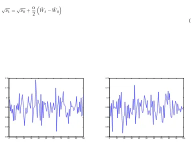
The price of a Call option is shown hereafter; but it is straightforward compute the value of a Digital option, or for example also of a cover warrant contract. We can observe that our model verifies the law of monotony according to volatility behaviour; in fact, if the volatility increases, the price increases too. Analogously, when the maturity dateT increases also the price in-creases; again, if the interest rate increases, we obtain that the option price is more high than before. This behaviour is corrected and it can be observed in a true market, making trading. It is worth noting that we obtain the same price for negative and positive sign of correlation factor. We want to observe that in our model(2)the volatility oscillates around the initial value of volatility√ν0, in fact we have:

√_ν

t=√ν0+

α

2

˜

Wt−W˜0

(15)

0 10 20 30 40 50 60 70 80 90 100 0.06

0.07 0.08 0.09 0.1 0.11 0.12

0 10 20 30 40 50 60 70 80 90 100 0.06

0.07 0.08 0.09 0.1 0.11 0.12

Table 1: At the money Call price forSt= 100,E = 100α= 0.1,ρ= 0.6

r νt T-t Value

0.03 0.01 6/12 4.3956

0.03 0.04 6/12 8.4123

0.03 0.09 6/12 11.8321

0.03 0.16 6/12 15.2633

0.03 0.25 6/12 18.6649

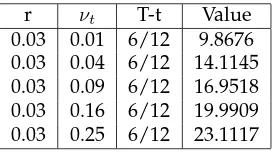
Table 2: In the money Call price forSt= 100,E= 90α= 0.1,ρ= 0.6

r νt T-t Value

0.03 0.01 6/12 9.8676

0.03 0.04 6/12 14.1145

0.03 0.09 6/12 16.9518

0.03 0.16 6/12 19.9909

0.03 0.25 6/12 23.1117

Table 3: Out the money Call price forSt= 100,E= 110α= 0.1,ρ= 0.6

r νt T-t Value

0.03 0.01 6/12 1.2788

0.03 0.04 6/12 4.6110

0.03 0.09 6/12 8.0435

0.03 0.16 6/12 11.5509

Table 4: At the money Call price forSt= 100,E = 100α= 0.1,ρ= 0.6

r νt T-t Value

0.07 0.01 12/12 7.1764

0.07 0.04 12/12 13.9619

0.07 0.09 12/12 18.6758

0.07 0.16 12/12 23.1458

0.07 0.25 12/12 27.7939

Table 5: In the money Call price forSt= 100,E= 90α= 0.1,ρ= 0.6

r νt T-t Value

0.07 0.01 12/12 11.4257

0.07 0.04 12/12 19.2650

0.07 0.09 12/12 23.5779

0.07 0.16 12/12 27.6163

0.07 0.25 12/12 31.9621

Table 6: Out the money Call price forSt= 100,E= 110α= 0.1,ρ= 0.6

r νt T-t Value

0.07 0.01 12/12 3.8234

0.07 0.04 12/12 9.002

0.07 0.09 12/12 14.6888

0.07 0.16 12/12 19.3951

5

Conclusions

References

(1) Andersen, L,. and J. Andreasen (2002), Volatile Volatilities, Risk Magazine, December.

(2) Andersen, L. and R. Brotherton-Ratcliffe (2005), Extended LIBOR market models with stochas-tic volatility, Journal of Computational Finance, vol. 9, no.1, pp. 1-40.

(3) Andersen, L. and V. Piterbarg (2005), Moment explosions in stochastic volatility models, Finance and Stochastics, forthcoming.

(4) Andreasen, J. (2006), Long-dated FX hybrids with stochastic volatility,Working paper, Bank of America.

(5) Broadie, M. and O . Kaya (2006), Exact simulation of stochastic volatility and other affine jump diffusion processes, Operations Research, vol. 54, no. 2.

(6) Broadie, M. and O . Kaya (2004), Exact simulation of option greeks under stochastic volatil-ity and jump diffusion models, in R.G. Ingalls, M.D. Rossetti, J.S. Smith and

(7) B.A. Peters (eds.), Proceedings of the 2004 Winter Simulation Conference.

(8) Carr, P. and D. Madan (1999), Option Pricing and the fast Fourier transform, Journal of Computational Finance, 2(4), pp. 61-73.

(9) Cox, J., J. Ingersoll and S.A. Ross (1985), A theory of the term structure of interest rates, Econometrica, vol. 53, no. 2, pp. 385-407.

(10) Duffie, D. and P. Glynn (1995), Efficient Monte Carlo simulation of security prices, Annals of Applied Probability, 5, pp. 897-905

(11) Duffie, D., J. Pan and K. Singleton (2000), Transform analysis and asset pricing for affine jump diffusions, Econometrica, vol. 68, pp. 1343-1376.

(12) Dufresne, D. (2001), The integrated square-root process, Working paper, University of Mon-treal.

(13) Glasserman, P. (2003), Monte Carlo methods in financial engineering, Springer Verlag, New York.

(15) Heston, S.L. (1993), A closed-form solution for options with stochastic volatility with appli-cations to bond and currency options, Review of Financial Studies, vol. 6, no. 2, pp. 327-343.

(16) Johnson, N., S. Kotz, and N. Balakrishnan (1995), Continuous univariate distributions, vol. 2, Wiley Interscience.

(17) Kahl, C. and P. Jackel (2005), Fast strong approximation Monte-Carlo schemes for stochastic volatility models, Working Paper, ABN AMRO and University of Wuppertal.

(18) Lee, R. (2004), Option Pricing by Transform Methods: Extensions, Unification, and Error Control, Journal of Computational Finance, vol 7, issue 3, pp. 51-86

(19) Lewis, A. (2001), Option valuation under stochastic volatility, Finance Press, Newport Beach.

(20) Lipton, A. (2002), The vol-smile problem, Risk Magazine, February, pp. 61-65.

(21) Lord, R., R. Koekkoek and D. van Dijk (2006), A Comparison of biased simulation schemes for stochastic volatility models, Working Paper, Tinbergen Institute.

(22) Kloeden, P. and E. Platen (1999), Numerical solution of stochastic differential equations, 3rd edition, Springer Verlag, New York.

(23) Moro, B. (1995), The full Monte, Risk Magazine, Vol.8, No.2, pp. 57-58.

(24) Patnaik, P. (1949), The non-centralχ2_{and F-distributions and their applications, Biometrika,}

36, pp. 202-232.

(25) Pearson, E. (1959), Note on an approximation to the distribution of non-centralχ2_{, Biometrika,}

46, p. 364.

(26) Piterbarg, V. (2003), Discretizing Processes used in Stochastic Volatility Models, Working Paper, Bank of America.

(27) Piterbarg, V. (2005), Stochastic volatility model with time-dependent skew, Applied Mathe-matical Finance.