Experimental Modelling and Identification of
Compressible Flow through Proportional Directional
Control Valves
Bashir M. Y. NOURI
1,*, Ma’ali B. Y. SAUDI
21Faculty of Engineering, An-Najah National University, P.O.Box 7, Nablus, West-Bank Palestine
2Faculty of Economics and Administrative Sciences, An-Najah National University, P.O.Box 7, Nablus, West-Bank Palestine *Corresponding Author: bnouri@najah.edu
Copyright © 2014 Horizon Research Publishing All rights reserved.
Abstract
This paper derives an empirical model of the air flow through a variable area orifice of a 5-port proportional valve, in function of pressures at the supply port and at the pneumatic cylinder, i.e. including the flow resistance of the connecting tubes and fittings, and the (quasi-static) valve’s driving voltage. Effects of nonlinear flow through the valve, air compressibility in cylinder chambers, system identification, numerical simulation and model validation experiments were conducted and compared with theoretical models showing very good agreement. This Experimental model can be used in simulation and control of high performance pneumatic servo positioning systems, with applications in robotics and modern pneumatic tube transportation systems.Keywords
Control Valves; Identification, Experimental, Compressible Flow; Mechatronic Systems1. Introduction
The nonlinear air mass flow rate through a proportional valve’s orifices is a basic control issue in pneumatic servo systems. The ideal isentropic mass flow rate equations of compressible fluids are based on the stagnation conditions (see [5] and [7] , that makes those equations valid only if the speed of a gas flow before an orifice is almost equal to zero. This is not the case for many usual system designs. The airflow through the orifices of a 5-port/ 4-way proportional valve cannot reach the critical conditions (choked flow conditions) and the flow factor (ψ) could be direction dependent. If there be, in addition, other flow resistance elements in the pneumatic circuit (e.g. tubes, bends, etc.).
In the past few decades, several researchers used mathematical models for compressible flow through the orifices of proportional valves. Some researchers derived mathematical models and assumed adiabatic charging and
discharging process, see [6], other researchers found experimentally that the temperature inside the chambers of pneumatic cylinder lays between the theoretical adiabatic and isothermal curves, see [1], and other researchers used mathematical models where they assumed that charging process is adiabatic and the discharging process is isothermal, see [4].
The most flexible and accurate servo performance can be achieved when a sufficiently fast proportional valve is used [11]. This is a necessary condition; an effective pressure-flow model is needed to complement this.
This paper derives an empirical model of the air flow through a variable area orifice of a 5-port proportional valve, in function of pressures at the supply port and at the pneumatic cylinder, i.e. including the flow resistance of the connecting tubes and fittings, and the (quasi-static) valve’s driving voltage. The model is derived with the aid of the test set-up described further in this paper.
Section 2 discusses the operation of the used 5/3-way proportional directional control valve. Section 3 discusses the model structure of the flow through the orifices of the proportional valve. Section 4 describes the used test set-up for deriving the valve flow equation. Section 5 derives an empirical model of the flow through the variable area orifice of the 5/3-way proportional directional control valve. Section 6 compares the actual proportional valve and its simulation model. Section 7 concludes the paper with some comments and statements.
2. Operation of a 5/3-Way Proportional
Directional Control Valve
The valve has 5-ports that are numbered from 1 through 5, such as shown in Fig 1. Air flow through the valve is controlled in magnitude and direction by the spool of the valve that is driven by an electromagnetic actuator (voice coil actuator). Thus, four orifices can be considered: the arrangements 1,2 and 1,4 are corresponding to charging orifices, i.e. charging air from an upstream air supply to downstream chambers, and the arrangements 2,3 and 4,5 are corresponding to discharging orifices, i.e. discharging air from downstream chambers to the atmosphere.
Figure 1(a & b). 5-Ports/ 3-way proportional directional control valve
The position of the spool is measured and the valve has a feedback system with a bandwidth of about 70 Hz. Thus, the spool’s position is proportional to the input voltage signal. The valve’s set-point voltage (u + Uref) range is 0 - 10 V DC. The valve is a voltage variation type, the central position (spool’s mid position) corresponds to Uref = 5 V, where the considered four orifices are closed. The driving voltage signal (u) has a range of - 5.0 to + 5.0 V DC.
With the aid of Figure 1, the operation of the valve can be listed in three cases as the following:
1. If the driving voltage (u) is zero and Uref = 5 V, then the spool of the valve is in its mid position where the considered four orifices are closed, but there will be leakage from the supply to the downstream chambers and to the atmosphere, Fig 2.
2. If the driving voltage (u) is increased gradually from 0 to 5.0 V, the spool of the
valve, see Fig 1, will
move starting from the mid position towards the
right hand side. During this motion, orifice 1,2
is opened for charging air from the supply to a
down
stream chamber, and orifice 4,5 is opened proportionally to orifice 1,2 for discharging air from a downstream chamber to the atmosphere. Orifices 1,4 and 2,3 will be closed, Fig 2.3. If the driving voltage (u) decreased gradually from 0
to -5.0 V, the spool of the valve, will move starting from the mid position towards the left hand side. During this motion, orifice 1,4 is opened for charging air from the supply to a downstream chamber, and orifice 2,3 is opened proportionally to orifice 1,4 for discharging air from a downstream chamber to the atmosphere. Orifices 1,2 and 4,5 will be closed, Fig 2.
Figure 2. The operation of the 5/3-way proportional directional control valve (FESTO, MPYE-5-1/8HF-010B).
The considered 5/3-way proportional directional control valve has a dead zone that is modelled by a dc voltage. The dead zone is asymmetric around the spool’s mid position, it is located between u+Uref = 4.252 V and 5.198 V, see Fig 2.
3. Model Structure for the Flow through
the Variable Area Orifice of the
5-Port Proportional Valve
[image:2.595.332.526.158.343.2]Consider the ideal nozzle that is shown in Fig 3. The gas flow is supplied from a large size chamber, where the stagnation conditions are assumed.
Figure 3. Isentropic flow through an ideal nozzle
One can step-by-step derive the equation of isentropic flow through the considered ideal nozzle and with aid of [ 5 ] and [ 7 ].The new general form of the ideal isentropic mass flow rate through a single ideal nozzle is given by:
)
P
/
P
(
)
,
T
,
R
(
C
P
A
m
=
eff 1 1κ
ψ
T 2 1 (1) [image:2.595.76.284.198.426.2] [image:2.595.379.495.553.645.2]1 1
1
1
,
)
R
T
2
(
1
)
2
1
T
,
R
(
C
κ−
+
κ
+
κ
κ
=
κ
(2)
and ≤ < ≤ < − − κ + κ +κ
= ψ κ + κ κ − κ crit 1 2 1 2 crit 1 1 2 2 1 2 1 1 T P P P 0 , 1 1 P P P , P P P P 1 1 2 1 (3)
Where:
m
: air mass flow rate, Aeff: effective flow area, ψT: air flow factor of an ideal nozzle, P: absolute pressure, T: absolute temperature, R: gas constant, κ: isentropic constant (ratio of specific heats), 1 and 2 indicates upstream and downstream respectively.The previous mass flow rate equations is based on the stagnation conditions, so the equations are valid only if the speed of the flow before the orifice is almost equal to zero, i.e. the cross-sectional area of the feeding tube is far bigger than that of the orifice. This is obviously not the case for many usual system designs, but nevertheless one can prove that the error introduced therein is acceptable. If the ratio of the tube cross-sectional area to the orifice cross-sectional area is 2 to 1, then the maximum introduced error by using the equation is less than 3.5 % [11].
Eq. 3 gives the flow factor graph that is depicted in Fig 4. In particular, the function ψT shows saturation behaviour for
P P
2/
1≤
P
crit corresponding to choked flow. In theunchoked regime (
P
crit<
P P
2/
1≤
1
), ψT is often approximated by the ellipse.ψ
TP P
b
b
=
−
−
−
1
1
2 1 2 [image:3.595.328.536.467.642.2]/
(4)
Figure 4. Ideal flow factor, ψ(P2/P1).
where, ideally,
b P
=
crit. It can easily be shown that theflow function for more than one orifice in series, taking P1 and P2 as the inlet and outlet pressures, will be different from that for a single orifice. In particular,
P
crit→
b
n , for n identical orifices.The ideal nozzle formula (Eq. 1) is used as qualitative basis for our model. For a single ideal orifice, there are two flow regimes: unchoked flow (
b P
=
crit>
05283
.
) and [image:3.595.86.268.517.720.2]choked flow (
b P
=
crit ≤ 0.5283) where the flow function ψT shows saturation behaviour. It can be easily shown with the aid of [ 5, and 7 ] that for more than one orifice in series, taking P1 and P2 as the inlet and outlet pressures, the flow factor will be different from that of a single orifice. In particular,P
crit→
b
n, for n identical orifices in series. Moreover the flow characteristic ψ could be direction dependent. If there are, in addition, other flow resistance elements in the pneumatic circuit (e.g. tubes, bends, etc.), Fig 5, it would be rather pointless to try to fit the experimental data with the ideal nozzle formula. On the other hand, it would be reasonable to expect that an empirical model would have the same structure as that of a series (of unknown number) of arbitrary orifices; i.e. the flow parameters and their combinations will remain basically unaltered. Our task boils down then to identifyingA
eff× ψ
( /
P P
2 1)
where 0 ≤ ψ ≤ 1 while retainingP
1×
C R T
( , , )
κ
, see Eq. 1. Further, if, for a given Aeff (proportional to the driving voltage |u|, Fig 5), ψ will saturate for a sufficiently small P2/P1, as is often the case in practice, it will then be possible and expedient to differentiate between the two terms Aeff and ψ, which would otherwise be lumped together.Figure 5. Schematic representation of the real pneumatic system
5. Experimental Test Set-up
tank (the supply) to the down stream tanks (tank 1 and tank 2, with volume of 30.27 litres each) representing the two sides of the pneumatic cylinder. The flow is governed in magnitude and direction by the position of the valve’s spool that is driven by an electromagnetic actuator (a solenoid). The downstream pressure in tanks 1 and 2 is measured by the pressure transducers for both charging and discharging operations; i.e. filling and emptying the tanks. A DSP-card that is installed in the computer, is used for providing the driving input voltage to the valve via a D/A converter and reading the pressure transducers via A/D converters.
6. Valve Flow Equation
A systematic series of experiments have been performed on the test set-up of Fig 6 to determine the flow rate through the orifices of the proportional valve as a function of the valve’s driving signal (representing the size of an orifice), and downstream and upstream pressures.
In these experiments, the valve is first set at its neutral position (spool’s mid position, Uref = 5 volt). Then, for a given spool DC voltage u, and supply pressure PS (or initial tank pressure respectively), the pressure variation in the tank that is being charged or discharged, is measured in real time (sampling time, tS = 0.10 sec). This was carried out for all combinations of drive voltage (|u| = 1, 2, 3, 4, and 5 volt), and supply pressure (PS = 1, 2, 3, 4, 5, 6, and 7 bar gauge pressure).
[image:4.595.130.510.257.637.2]During a charging or a discharging process, the mass flow rate is obtained by differentiating, w. r. t. time, the equation of state of the air contained in the known control volume (volume of the tank). For simplicity and since only an empirical model is sought for, the process is assumed isothermal throughout, i.e. T = Tref = Tatm. Hence, we have
P V
=
m R T
(5)where V, R and T are constants (V = volume of a tank, P = absolute pressure in the tank, T = absolute room temperature, and m = mass of air in the tank).
Differentiating Eq. 5 and rearranging yields:
m
V
R T
P
=
(6)That is to say that the mass flow rate can be obtained by differentiating the tank-pressure measurements in the time. In practice,however, since direct differentiation of the (noisy) experimental data can be quite cumbersome, creative identification techniques have been devised to validate the models and quantify their parameters as will be sketched in the following:
First of all, the valve effective orifice area Aeff, as a function of the valve driving voltage and the upstream pressure, can be identified, up to a constant factor, as follows:
Since, for a given constant upstream pressure, the downstream pressure satisfies
~
( )
P
A
effψ
P
(7) then, separating the variables P and t and integrating yields:F P d P
P Aeff d t A teff
( )
( ) ~
=
∫
∫
=ψ (8)
[image:5.595.343.531.78.238.2]This function, F, represents the tank pressure evolution that is measured in the experiment, Fig 7. The result means that, for a fixed upstream pressure, the downstream pressure evolution should have the same form when the time axis is scaled by a factor proportional to the effective area, Fig 8.
Figure 7. Measured downstream pressure evolution in tank 1. Charging through orifice 1,4 at constant supply gauge pressure of 7 bar and for three set point driving voltages (|u| = 1, 2, and 3 volt).
Figure 8. Result of scaling the time axis of the measured downstream pressure evolution in tank 1. Charging through orifice 1,4 at constant supply gauge pressure of 7 bar and for three set point driving voltages (|u| = 1, 2, and 3 volt). The pressure evolution corresponding to the driving voltage |u| = 1.0 volt is the reference.
Thus, for a group of tank pressure evolution curves corresponding to the same upstream pressure, a best fit of those curves is sought onto one another using the scaling factors as fitting parameters. In this way (i) the dependence of the effective area on the valve driving voltage and the supply pressure is determined and (ii) a single best fit is sought for the whole group, which is then used to identify the flow factor, ψ.
Summing up, the mass flow rate through the valve is modelled by the formula
( )
( ) ( / )
m A P
RT P P
eff = ± + + − 1 1 1 2 1 2 1 2 1 κ
κ κ ψ
κ (9)
where, ± indicates charging or discharging respectively, and P1 is the absolute upstream pressure. Aeff and ψ are to be experimentally identified.
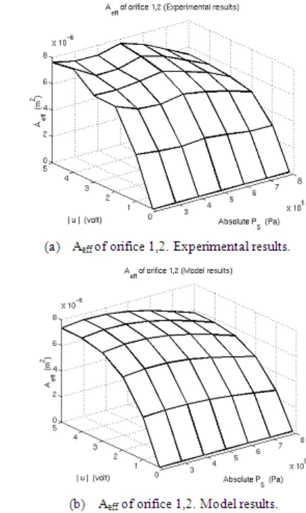
As regards the effective orifice area for each orifice of the valve that is modelled by Eq. 10, the identification results show that it is primarily a function of the driving voltage and, to a lesser extent, the supply pressure as shown in Fig 9, 10, 11 and 12.
A A u U U U P P eff m S o S C D
S S o
= − − − + + 1
2 2 1
α α α (10)
[image:5.595.88.270.564.722.2]Since the considered 5/3-way proportional directional control valve has four orifices, see section 1, the parameters of the effective orifice area’s model are identified for every orifice independently from the others.
Table 1 shows the identified effective area model parameters for the considered valve’s four orifices.
[image:5.595.367.509.577.626.2]of the flow, that has been alluded to earlier, but also from the fact that, for discharging, an extra flow resistance element has been added at the outlet; viz. a silencer to subdue exhaust noise. These two functions are given by:
Charging:
ψ
β γ
C S
P
P b
b
= −
−
−
1
1 2
(11)
Discharging:
ψD n atm
n
n n
A P
P
=
=
=
∑
20 12
[image:6.595.309.530.82.452.2](12)
Figure 9. Experimental and modelled values for the effective area of the charging orifice 1,4.
[image:6.595.332.532.495.662.2]Figure 11. Experimental and modelled values for the effective area of the discharging orifice 2,3.
Figure 12. Experimental and modelled values for the effective area of the discharging orifice 4,5.
Table 1. Identified model parameters of the valve’s effective
Charging Discharging
Parameter Orifice 1,4 Orifice 1,2 Orifice 4,5 Orifice 2,3 Am
[ m2 ] 7.302*10-6 7.566*10-6 11.96*10-6 11.71*10-6
C
[ ] 3.4174 3.1949 3.3361 3.8045 D
[ ] 0.9628 0.9721 1.1522 1.1038 α2
[Pa-2] 1.88*10-12 1.46*10-12 -4.64*10-13 -3.39*10-13
α1
[Pa-1] -1.40*10-6 -0.99*10-6 9.99*10-7 9.06*10-7
αo
[ ] 1.238 1.167 0.824 0.827
Uo
[volt] 0.748 0.198 0.198 0.748
US
[volt] 5.000 5.000 5.000 5.000
[image:7.595.309.551.86.286.2]Eq. 11 has the same general form as Eq. 4, where the parameter b is the critical (saturation) pressure ratio. Identification shows that β = 8.0682, γ = 0.8550, and b = - 0.6682. Negative critical pressure ratio means that the flow never saturates (or “chokes”).
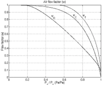
Table 2 shows the identified parameters of the discharging flow factor’s model, ψD. For the purpose of comparison, Fig 13 plots the theoretical air flow factor, for a single ideal nozzle ψT, together with those experimentally identified for charging ψC and the discharging ψD, respectively.
Figure 13. Comparison between ψT, ψC and ψD air flow factors.
6. Simulation of the 5/3-Way
Proportional Directional Control
Valve
In order to establish conformity of behaviour with practice and gain some idea about the general behaviour, a simulation model for the experimental test set-up, Fig 6, is constructed by using SIMULINK and MATLAB workspace.
P
R T
V
m d t
P
o [image:7.595.76.279.313.475.2] [image:7.595.345.520.422.566.2] [image:7.595.74.278.520.700.2]For the purpose of comparison between the simulation scheme and the real used test set-up, the measured and simulated pressures in a downstream tank are compared for a given set point driving voltage and supply pressure, see Fig 14 and 15. These figures show that there is a good correspondence between the measured and the simulated downstream pressures.
Table 2. The coefficients of the discharging air flow factor, ψD
N An
0 - 3.6047
1 154.1813
2 - 2275.8988
3 19553.9533
4 - 108731.1339
5 412066.8918
6 - 1093022.8206
7 2049011.9540
8 - 2700562.9401
9 2446283.6714
10 - 1449043.8060
11 505075.9974
12 - 78506.4234
The minor deviations come from the single best fit of a group of a downstream tank pressure evolution curves corresponding to the same upstream pressure after scaling the time axis by a factor proportional to the effective area, see Fig 8.
The minor deviations could also come from some unavoidable experimental errors, such as small variations in the supply pressure during some of the experiments.
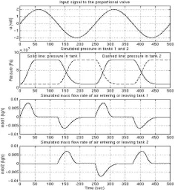
Its influence on the experiments is apparent in the experimentally identified effective area, see Fig 10-a. For testing the validity of the proportional valve’s model (model of compressible flow through a variable area orifice), a sinusoidal input signal is given, and the simulated downstream pressures (pressures in tanks 1 and 2) and air mass flow rate through the considered four orifices are recorded. That is done for two cases (i) proportional valve without dead zone compensation, Fig 16 and (ii) proportional valve with dead zone compensation, Fig 17.
The simulation results show that the model of the valve that is represented by an m-File using MATLAB software can be used for simulating actual proportional directional control valves operated under various conditions.
[image:8.595.339.510.464.632.2]Figure 15. Measured pressure (solid line) and simulated pressure (dashed line) in tank 2, respectively. Charging through orifice 1,2 and discharging from tank2 to the atmosphere through orifice 2,3.
Figure 16. Simulated pressure and mass flow rate without valve’s dead zone compensation.
Figure 17. Simulated pressure and mass flow rate with valve’s dead zone compensation.
7. Conclusions
An essential element, that is characterized by a nonlinear behaviour, of a pneumatic servo positioning system has been identified and modelled effectively.
The servo valve’s driving voltage-pressure-flow relation is identified and modelled based on the single nozzle model structure. Although the latter proved sufficient for modelling/ identification purpose, the form of the flow-pressure function actually obtained significantly departs from the nozzle formula that is commonly used for modelling servo valves. Moreover, two different functions have been obtained for charging to the cylinder and discharging to atmosphere, respectively, such might be important for accurate control design.
Creative identification techniques have been devised to validate the models and quantify their parameters. A simulation model of the pneumatic servo valve is constructed and compared with the real valve showing good agreement.
REFERENCES
[1] Al-Ibrahim, A.M., and Otis, D.R., 1992, Transient Air Temperature and Pressure Measurements During the Charging and Discharging Processes of an Actuating Pneumatic Cylinder, Proceedings of the 45th National Conference on Fluid Power, 1992.
[2] Andersen, B., 1967, The Analysis and Design of Pneumatic Systems, New York, John Willey & Sons, Inc.
[3] Burrows, C.R., and Webb, C.R., 1966, Use of the root Loci in Design of Pneumatic Servo-Motors, Control, Aug., pp. 423-427.
[4] Edmond Richer and Yildirim Hurmuzlu, 2000, A High Performance Pneumatic Force Actuator System: Part 1-Nonlinear Mathematical Model. ASME Journal of Dynamic Systems Measurement and Control, Vol. 122, No.3, pp. 416-425
[5] Fox, Robert W., and Alan T. McDonald (2008). Introduction to fluid mechanics. Seventh Edition, John Willey & Sons, INC.
[6] Liu, S., and Bobrow, J.E., 1988, An Analysis of a Pneumatic Servo System and Its Application to a Computer-Controlled Robot, Journal of Dynamic Systems, Measurement, and Control, Vol. 110, pp. 228-235.
[7] Munson, B.R., Young, D.F., and Okiishi, T.H., 1999, The Fundamentals of Fluid Mechanics. Third Edition, John Willey & Sons, New York.
[8] Richard E., Scavarda, S., 1996,Comparison Between Linear and Nonlinear Control of an Electropneumatic Servodrive, Journal of Dynamic Systems, Measurement, and Control, Vol. 118, pp. 245-118.
[image:9.595.89.265.311.508.2] [image:9.595.89.268.543.735.2][10] Shearer J. L. (February, 1957). Nonlinear analog study of high-pressure pneumatic servomechanism. Transactions of the ASME, pp. 465-472.