Transient Stability Analysis of SMIB System Equipped with Hybrid Power Flow Controller

(1)

International Journal of Emerging Technology and Advanced Engineering

Website: www.ijetae.com (ISSN 2250-2459, Volume 2, Issue 2, February 2012)

18

Transient Stability Analysis of SMIB System Equipped

with Hybrid Power Flow Controller

Lini Mathew

1

, S.Chatterji

2

1,2 _{Electrical Engineering Department, NITTTR, Chandigarh, India}

lenimathew@yahoo.com chatterjis@yahoo.com

Abstract—Recently, a novel hybrid power flow controller (HPFC) topology for FACTS was proposed. The key benefit of the new topology is that it fully utilizes existing equipment. The MATLAB/SIMULINK models of three different configurations of HPFC have been investigated for their different characteristics, by incorporating them in the SMIB system. In all the three cases, the steady state stable values of rotor-angle, time taken to attain stability, maximum overshoot and the rise-time by varying the FCT, and also by varying the damping constants, have been found out. Any of these configurations can effectively be incorporated in a SMIB system and contributes highly in the transient stability enhancement of the system

Keywords— Hybrid Power Flow Controller (HPFC), FACTS, MATLAB/SIMULINK, SMIB System, Transient Stability

I. INTRODUCTION

FACTS controllers refer to devices that enable flexible electrical power system operation, in the way of controlled active and reactive power flow redirection in transmission paths, by means of flexible and rapid control over the ac transmission parameters [1]. FACTS Controllers can be classified as (i) variable impedance type controllers and (ii) voltage source converter based controllers. Thyristor switches (formed by way of connecting two thyristors in anti-parallel) are connected in series or in shunt along with reactors or capacitors to form thyristor based variable impedance type FACTS Controllers. Such controllers are employed for controlling the reactive power in the system [2]. Static Var Compensator (SVC), Thyristor-Controlled Series Capacitor (TCSC), are some of the examples of such FACTS Controllers.

The basic building block of a Voltage Sourced Converter (VSC) is a three-phase converter bridge. When a VSC is interfaced with a transmission system, it can vary the magnitude and the phase-angle of its output voltage with respect to the system voltage and thus, exchange active and reactive power with the transmission system.

Static Synchronous Compensator (STATCOM), Static Synchronous Series Compensator (SSSC), Unified Power Flow Controller (UPFC), Interline Power Flow Controller (IPFC) etc. are the well-known VSC based FACTS Controllers.

The considerable price of VSC based FACTS Controllers remains the major impediment to their widespread use, even though these devices lead to reduction in the equipment size and also improved performance. The existing classical equipment such as the switched capacitors and the SVC used for voltage support and switched series capacitors and TCSC used for line impedance control need to be replaced whenever system upgradation or performance improvements are planned. The main disadvantage of the topology of UPFC is that the device is entirely converter based. It uses the shunt converter to supply the active power coupled with the series converter, and once the shunt converter is in place, it is also used to supply the required reactive power [3]. The UPFC can make limited use of the existing classical equipment.

Environmental, right-of-way and cost problems have over the years, limited construction of both generation facilities as well as new transmission lines. Better utilization of existing power systems along with effective control equipment has thus, become imperative. This creates a situation wherein novel and cost effective FACTS topologies are required to be built upon the existing equipment. This establishes the use of static converters.

II. HYBRID POWER FLOW CONTROLLER

(2)

International Journal of Emerging Technology and Advanced Engineering

19

The key benefit of this new topology is that, it fully utilizes the existing equipment such as switched capacitors or SVC etc. and thus the required rating of the additional converter is substantially lower as compared to the rating of the comparable UPFC.

The Hybrid Power Flow Controller (HPFC) uses two equally rated voltage sourced converters in order to upgrade the functionality of the existing switched capacitors or Static VAR Compensators (SVC). Recently, a novel HPFC topology for FACTS was proposed. It consists of a shunt connected controllable source of reactive power, along with two series connected voltage sourced converters – one on each side of the shunt device. The converters can exchange active power through a common dc circuit. A block diagram representation of such an envisioned typical HPFC application is shown in Fig.1.

This HPFC configuration is assumed to be installed on a transmission line that connects two electrical areas ie. on a Single Machine Infinite Bus (SMIB) System. Central to the HPFC topology is the shunt connected source of reactive

power denoted as BM and represents the controllable shunt

connected variable capacitance. This is equivalent to a typical SVC or any other functional equivalents of SVC such as STATCOM, a synchronous condenser or even a mechanically switched capacitor bank. The two voltage

sourced converters VSCx and VSCY, are connected to the

transmission line by means of coupling transformers. The converters provide controllable voltages at terminals of high voltage side of the transformers. The converters share a common dc circuit coupling each others’ dc terminals. The dc circuit permits exchange of active power between the converters [5]. The flow of active power through the line and the amounts of reactive power supplied to each line segment can be simultaneously and independently controlled by varying the magnitudes and the phase-angles of the voltages supplied by the converters.

Control of the shunt connected reactive element is coordinated with the control of converters to supply the bulk of the total required reactive power.

The hybrid power flow controller is installed on a transmission line dividing it into two transmission line segments. This is shown in Fig.1. The line to neutral voltage at the point of connection of the hybrid power flow

controller with one line segment is denoted by V1. The

voltage at the point of connection of the other line segment

to the HPFC is denoted by V2. The three-phase

transmission line segments are carrying three-phase

alternating currents denoted as IS and IR. A simplified

single-phase equivalent of the circuit of the system shown in Fig.1 has been depicted in Fig.2.

The voltage sources VX and VY shown in Fig.2 represent

the high voltage equivalents of voltages generated by the

voltage source converters VSCX and VSCY respectively.

BM represents the controllable shunt connected variable

susceptance. Active and reactive powers of the converters

are shown by PX, QX, PY, and QY respectively [4].

When switching functions are approximated by their fundamental frequency components neglecting harmonics, HPFC can be modeled by transforming the three phase voltages and currents to dq0 variables using Park’s transformation which is given by:

VDQ0 = T Vabc --- (1)

where,

--- (2) V1

V2

VX _V_Y

IS IR

IM

~

VR VS

VM

BM

ZS ZR

CDC VD

C

PX _P_Y

PX, QX PY, QY

HPFC

VS VR

~

CDC VSCY

VSCX

VM

BM

V1 V2

Fig.1 SMIB System incorporated with a HPFC Controller in the Power System

(3)

International Journal of Emerging Technology and Advanced Engineering

20

The two voltage source converters connected in series

are represented by controllable voltage sources VX and VY .

VM is the voltage at the point where the variable

susceptance is connected. LR, LS, RR, RS are inductances

and resistances of transmission line of both sides of HPFC.

PX is the real power exchange of the converter VSCX with

the dc link and PY is the real power exchange of the

converter VSCY with the dc link. At any instant of time,

PX = PY --- (3)

The shunt connected variable susceptance or capacitance has been modeled by means of the differential equations given by: Rd Sd Md Mq M Md M I _ I = I = V B + dt dV ω B

--- (4) Rq Sq Mq Md M Mq M I _ I = I = V B + dt dV ω B --- (5)

The model of the series converter VSCX and the line

segment on the sending end is given by:

Sd Md Xd Sd S Sq S Sd

S +ωL I +R I +V +V = V

dt dI L --- (6) Sq Mq Xq Sq R Sq S Sq

S +ωL I +R I +V +V =V

dt dI L

--- (7) The differential equations describing the dynamics of the

series converter VSCY and the line segment on the

receiving end are given by:

Rq R Yd Md Rd Rd R Rd

R +R I +V =V +V +ωL I

dt dI L --- (8) Rd R Yq Mq Rq Rq R Rq

R

_dt

+

R

I

+

V

=

V

+

V

+

ω

L

I

dI

L

--- (9)

The differential equation describing the dynamics of Vdc is

given by:

(

_X _Y

)

dc dc

dc _V P _P

1 = dt dV

C --- (10)

The dc circuit permits the exchange of active power between the converters [6].

HPFC can be used to control simultaneously and independently the flow of active power through the line and the amounts of reactive power exchanged with the sending end and the receiving end. HPFC can thus be regarded as the functional equivalent of UPFC. The influence of HPFC on power system stability mainly the transient stability, has been investigated in the following sections.

III. MATLAB/SIMULINK BASED MODEL OF SMIBSYSTEM

EQUIPPED WITH HYBRID POWER FLOW CONTROLLER

The hybrid power flow controller shown in Fig.1 consists of two power converters connected in series. In order to divert the current, a controllable susceptance is connected as shunt at a nodal point between the converters. The MATLAB/SIMULINK model of such an arrangement is shown in Fig.3. It consists of two 100 MVA, three-level, 48-pulse GTO based converters, connected in series. The series converters are interconnected through a dc bus. An SVC is connected as shunt at a nodal point between the first and second converter. The SVC consists of a 230kV/16 kV 333 MVA coupling transformer, thyristor-controlled reactor (TCR) and thyristor-switched capacitor (TSC) banks. The above configuration has been named as HPFCD1 by the authors and has been incorporated in the SMIB system.

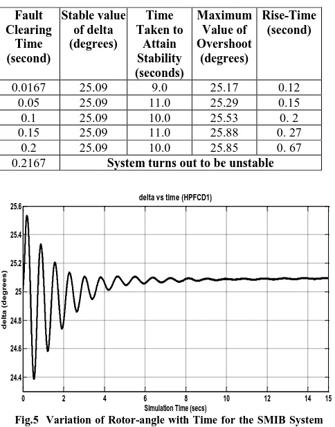
The SMIB system equipped with HPFCD1 has been modelled and simulated using SimPowerSystems Library of MATLAB/SIMULINK for the purpose of investigating the characteristics of this particular configuration of HPFC, and is as shown in Fig.4. The HPFCD1 is located at the sending end of the line between buses B1 and B2. A three-phase fault has occurred at the receiving end of the transmission line. The fault clearing time (FCT) is considered to be 0.1s. The stable value of rotor-angle, time taken to attain stability, maximum overshoot and the rise-time, for different values of fault clearing time (FCT) are tabulated in Table I.

(4)

International Journal of Emerging Technology and Advanced Engineering

21

[image:4.612.51.290.138.275.2]

It is observed from Table I that as the FCT increases, the values of maximum overshoot and the time taken to reach the maximum overshoot (rise time) also increase, but the stable value of the rotor angle and the settling time remain almost the same. Fig.5 shows the variation of rotor-angle () with time for the above SMIB system.

TABLE I

STABLE VALUE OF ROTOR-ANGLE, TIME TAKEN TO ATTAIN STABILITY, MAXIMUM VALUE OF OVERSHOOT, RISE-TIME FOR

DIFFERENT VALUES OF FAULT CLEARING TIMES Fault

Clearing Time (second)

Stable value of delta (degrees)

Time Taken to

Attain Stability (seconds)

Maximum Value of Overshoot (degrees)

Rise-Time (second)

0.0167 25.09 9.0 25.17 0.12 0.05 25.09 11.0 25.29 0.15 0.1 25.09 10.0 25.53 0. 2 0.15 25.09 11.0 25.88 0. 27

0.2 25.09 10.0 25.85 0. 67 0.2167 System turns out to be unstable

0 2 4 6 8 10 12 14 15

24.4 24.6 24.8 25 25.2 25.4 25.6

Simulation Time (secs)

d

e

lt

a

(

d

e

g

r

e

s

)

delta vs time (HPFCD1)

The locations of HPFCD1 and the three-phase fault have been changed and the above values have been compared in all the cases. The system behaves almost in the same manner, except some minor changes in the values. The critical clearing time (CCT) in all these cases have been found out. It is obvious that a FCT more than the CCT, will cause the system to be unstable. The values of CCT for different locations of fault and the placement of HPFCD1 are shown in Table II.

TABLE II

VALUES OF CCT FOR DIFFERENT LOCATIONS OF HPFCD1 AND POINTS OF OCCURRENCES OF FAULT

Placement of HPFCD1

Values of CCT when the point of occurrence of fault is at

Sending end Mid point Receiving end

Sending end 0.233 0.2 0.2

Mid point 0.233 0.083 0.15

Receiving end 0.233 0.1 0.15

[image:4.612.50.292.415.723.2]

The system has again been analyzed by varying the damping constants. Table III shows the stable value of rotor-angle, time taken to attain stability, maximum overshoot and the rise-time, for various values of damping constant.

TABLE III

DIFFERENT VALUES OF DAMPING CONSTANT

Damping Constant

Stable value of

rotor-angle (degrees)

Time Taken to Attain Stability (seconds)

Maximum Value of Overshoot

(degrees)

0.0 Sustained oscillations from 5s onwards

25.77 0.25

25.64 0.23

0.2 25.09 10.0 25.53 0.2 0.3 25.03 10.0 25.45 0.18 0.4 24.95 9.0 25.38 0.17 0.5 24.88 8.5 25.31 0.15 0.6 24.81 8.0 25.26 0.14 0.7 24.74 7.0 25.21 0.13 0.8 24.67 6.5 25.17 0.12 0.9 24.60 6.0 25.14 0.11 1.0 24.54 5.5 25.11 0.10 1.1 24.47 5.0 25.08 0.09 1.2 24.41 5.5 25.07 0.07 1.3 24.35 6.0 25.06 0.06 1.4 24.3 6.0 25.05 0.05 1.5 System turns out to be unstable

Fig.4 MATLAB/SIMULINK Model of SMIB System Equipped with HPFCD1

[image:4.612.261.553.461.710.2] [image:4.612.328.565.467.705.2]

(5)

International Journal of Emerging Technology and Advanced Engineering

22

It is observed from Table III that for lower values of damping constants, such as 0.0 and 0.1 the system exhibits sustained oscillations from 5 seconds onwards, For the system to attain stability the damping constant may be increased to 0.2. It is also seen that the stable values of rotor-angle, the time taken to attain stability, the maximum overshoot and the rise-time all decrease with an increase in the value of damping constant. For a value of damping constant of 1.5, the system turns out to be unstable.

IV. MATLAB/SIMULINK BASED MODEL OF THE SECOND

CONFIGURATION OF HYBRID POWER FLOW CONTROLLER

(HPFCD2)

The previous configuration of HPFC, named as HPFCD1, employed a typical SVC in place of the variable susceptance. It is apparent that functional equivalents of an SVC, such as a mechanically switched compensator bank, or a STATCOM can be successfully employed. The authors have designed another configuration using the above principle by replacing the SVC by a shunt compensator. The MATLAB/SIMULINK model of such an arrangement with two converters connected in series and a shunt compensator connected at the nodal point between the converters is shown in Fig.6.

A capacitive reactive power of 10 MVAR has been connected as the shunt compensator. The above configuration has been named as HPFCD2 and has been incorporated in the SMIB system for investigating its characteristics. The SMIB system equipped with HPFCD2 has been modelled and simulated using SimPowerSystems Library of MATLAB/SIMULINK.

A three-phase fault has been considered occurring at the receiving end of the transmission line and the HPFCD2 has been assumed to be located at the sending end of the line between buses B1 and B2. The fault clearing time (FCT) has been considered to be 0.1s. The variation of rotor-angle () with time for the above SMIB system is almost similar to the one shown in Fig.5.

[image:5.612.324.561.315.415.2]

The stable value of rotor-angle, time taken to attain stability, maximum overshoot and the rise-time, for different values of fault clearing time (FCT) are tabulated in Table IV. The values are almost same as the case shown in Table I.

TABLE IV

DIFFERENT VALUES OF FAULT CLEARING TIME

Fault Clearing

Time (second)

Stable value of delta (degrees)

Maximum Overshoot

(degrees)

0.0167 25.08 10.0 25.27 0.18 0.05 25.08 10.0 25.42 0.2

0.1 25.08 9.5 25.77 0.25 0.133 25.08 10.0 26.19 0.35

0.15 unstable

The locations of placement of HPFCD2 and the three phase fault have been changed to sending end, midpoint and receiving end of the transmission line and similar analysis have been carried out. The critical clearing time (CCT) in all these cases has been tabulated as in Table V.

TABLE V

Location of HPFCD2

Sending end 0.2 0.15 0.133

Mid point 0.2 0.067 0.1167

Receiving end 0.2 0.1 0.133

Comparing the Tables II and V, it is seen that the value of CCT is high when the fault occur at the sending end of the line. The system exhibits a low value of CCT when both HPFCD2 and the fault are located at the midpoint of the line.

[image:5.612.53.293.424.611.2]

The same system has further been analyzed by varying the value of damping constant. Table VI shows the stable value of rotor-angle, the time taken to attain stability, the maximum overshoot and the rise-time, for different damping constants.

(6)

International Journal of Emerging Technology and Advanced Engineering

23

TABLE VI

STABLE VALUEOF ROTOR-ANGLE, TIME TAKENTO ATTAIN

STABILITY, MAXIMUM VALUEOF OVERSHOOT, RISE-TIME FOR

DIFFERENT VALUESOF DAMPING CONSTANT

It is observed from Table VI that the system attains stability faster for a higher value of damping constant. If the damping constant is further increased, the settling time increases slightly, and the system becomes unstable at a damping constant value of 1.6. It is also observed that the steady state stable value of delta, the maximum overshoot and the rise-time decrease with increasing values of damping constant.

V. MATLAB/SIMULINK BASED MODEL OF THE THIRD

CONFIGURATION OF HYBRID POWER FLOW CONTROLLER

(HPFCD3)

The authors in this article, have devised another configuration of HPFC using STATCOM in place of SVC as used in case of HPFCD1. The MATLAB/SIMULINK model of such an arrangement with two converters connected in series and a STATCOM connected at the node between the converters is shown in Fig.7. The above configuration has been named as HPFCD3 and has been incorporated in the SMIB system for investigating its characteristics. The SMIB system equipped with HPFCD3 has been modelled and simulated using SimPowerSystems Library of MATLAB/ SIMULINK.

The HPFCD3 has been located at the sending end of the line between buses B1 and B2. The variation of rotor-angle () with time for the above SMIB system is again found to be similar as shown earlier for HPFCD1 in Fig.5

[image:6.612.333.577.133.339.2]

The stable value of rotor-angle, time taken to attain stability, maximum value of overshoot and the rise-time, for different values of fault clearing time (FCT) are given in Table VII. It can be observed from Table VII that HPFCD3 also exhibits similar properties as that of HPFCD1 and HPFCD2.

TABLE VII

DIFFERENT VALUES OF FAULT CLEARING TIME

Fault Clearing

Time (second)

Stable Value of delta (degrees)

0.0167 24.95 10.0 25.18 0.13 0.05 24.96 9.5 25.29 0.15 0.1 24.96 9.0 25.5 0.2 0.15 24.96 8.5 25.8 0.26

0.2 24.96 8.5 26.4 0.5

0.2167 unstable

The locations of HPFCD3 and the three-phase fault have been changed for analyzing the system behavior. It is found that the value of CCT for all these cases are different. The values of CCT for different locations of fault and HPFCD3 have been tabulated in Table VIII.

Stable value of

rotor-angle (degrees)

0.0 25.08 11.0 25.76 0.25 0.1 25.03 10.0 25.63 0.22 0.2 24.97 9.0 25.53 0.2 0.3 24.92 8.0 25.45 0.18 0.4 24.86 7.0 25.38 0.17 0.5 24.81 6.5 25.32 0.15 0.6 24.76 6.5 25.26 0.14 0.7 24.70 6.0 25.22 0.13 0.8 24.64 6.0 25.18 0.13 0.9 24.59 6.0 25.14 0.12 1.0 24.54 6.0 25.11 0.11 1.1 24.49 6.5 25.08 0.09 1.2 24.44 6.5 25.07 0.07 1.3 24.39 6.5 25.06 0.05 1.4 24.34 7.0 25.05 0.05 1.5 24.3 7.0 25.05 0.04 1.6 System turns out to be unstable

Fig.7 MATLAB/SIMULINK Model of the Third Configuration

[image:6.612.324.560.525.636.2]

(7)

International Journal of Emerging Technology and Advanced Engineering

24

TABLE VIII

Location of HPFCD3

Sending end 0.2 0.167 0.2

Mid point 0.083 0.1 0.183

Receiving end 0.233 0.1167 0.15

[image:7.612.325.564.198.411.2]

The above system has again been analyzed by varying the damping constants. The steady state stable value of rotor-angle, time taken to attain stability, maximum value of overshoot and the rise-time, for varying the value of damping constant have been tabulated in Table IX. Comparing Tables III and IX, it is found that the system exhibits sustained oscillations when it is incorporated with HPFCD1 or HPFCD3. In case of HPFCD2, it is different. In all the three cases the steady state stable value of rotor-angle, time taken to attain stability, maximum value of overshoot and the rise-time, for varying the value of damping constant are almost similar and same. It is found that the system attains stability faster as the value of damping constant increases.

TABLE IX

DIFFERENT VALUES OF DAMPING CONSTANT

The delta vs time plot of the three configurations of HPFC (HPFCD1, HPFCD2, HPFCD3) and UPFC is drawn in one figure for comparison purpose, and is shown in Fig.8. It is observed from Fig.8 that HPFCD1, HPFCD2 and HPFCD3 settles down almost at the similar values.

0 3 6 9 12 15

24.4 24.6 24.8 25 25.2 25.4 25.6 25.8 26

Simulation Time (secs)

delta

(deg

ree

s)

HPFCD1

HPFCD2

HPFCD3 UPFC

The above analysis reveals that any of the above explained three configurations can effectively be incorporated in SMIB system. They contribute much in the transient stability enhancement of the system. It can thus be concluded that HPFC performs effectively in damping of oscillations as compared to UPFC and other FACTS controllers, and the system is able to regain its stable post fault equilibrium point quite effectively and efficiently.

The authors in all the three above mentioned configurations of HPFC have employed the discrete solution method available in SimPowerSystems software. When simulating larger systems such as systems containing large number of states or non-linear blocks, or systems using power electronic devices like IGBT, GTO, FET etc, it is always advantageous to discretize the system. Such systems tend to become very precise, but slow.

VI. CONCLUSION

Three different configurations of HPFC based on the proposed concept have been simulated employing the discrete solution method available in SimPowerSystems software of MATLAB. The effectiveness of HPFC for enhancing the transient stability of power system has been analytically investigated for different conditions.

Stable Value of

Rotor-angle (degrees)

25.74 0.25

25.61 0.22

0.2 24.96 11.0 25.51 0.2 0.3 24.91 9.0 25.42 0.3 0.4 24.86 8.0 25.36 0.4 0.5 24.80 7.0 25.30 0.5 0.6 24.75 6.0 25.26 0.6 0.7 24.70 7.0 25.21 0.7 0.8 24.64 6.5 25.18 0.8 0.9 24.59 6.5 25.14 0.9 1.0 24.54 6.5 25.11 1.0 1.1 24. 48 6.5 25.09 1.1 1.2 24. 44 7.0 25.08 1.2 1.3 24. 38 7.0 25.07 1.3 1.4 24. 34 7.0 25.06 1.4 1.5 System turns out to be unstable

[image:7.612.47.285.447.691.2]

(8)

International Journal of Emerging Technology and Advanced Engineering

25

The simulation results are very encouraging and indicate that all the three configurations of HPFC considered in this article, help in improving the transient stability of power system. The investigations reveal that a power system equipped with HPFC stabilizes quickly, reduces the settling time, thus damps out the power system oscillations effectively. HPFC is found out to be almost similar to UPFC and superior to other FACTS controllers.

References

[1] Hingorani N.G., Gyugyi L, Understanding FACTS concepts and technology of Flexible AC Transmission Systems, IEEE Press, New York, 2000.

[2] Glanzmann.G., ―FACTS Flexible Alternating Current Transmission Systems‖, EEH – Power Systems Laboratory, ETH Zurich, January 2005.

[3] Bebic.J.Z., ―The Hybrid Power Flow Controller-Introduction to HPFC‖, Available at http://www.hpfc.ca/hpfc.html

[4] Bebic.J.Z., Lehn.P.W., Iravani.M.R., ―The Hybrid Power Flow Controller A New Concept for Flexible AC Transmission‖, Proceedings of the IEEE Power Engineering Society General Meeting, pp 1-7, June, 2006.

[5] Sood.V.K., Sivadas.S.D., ―Simulation of Hybrid Power Flow Controller‖, IEEE 2010.