Evolutionary Algorithms in Astrodynamics

ISSN Online: 2161-4725 ISSN Print: 2161-4717

Evolutionary Algorithms in Astrodynamics

Marcin Misiak

UAM, Poznan, Poland

Abstract

This paper presents the method of solving the equations of motions by evolutionary algorithms. Starting from random trajectory, the solution is obtained by accepting the mutation if it leads to a better approximations of Newton’s second law. The gen-eral method is illustrated by finding trajectory to the Moon.

Keywords

Genetic Algorithms, Newton’s Equations of Motion, Principle of Least Action, Astrodynamics, Celestial Mechanics, Orbital Motion, Optimal Control, Two-Point Boundary Value Problem

1. Introduction

In this paper, we examine the application of a simple evolutionary algorithm with mu-tation only (no recombination) for solving general dynamical problems resulting from Newton’s second law and will use it to solve the special astrodynamical problem, namely finding the trajectory to the Moon.

In the last decades, there is a growing interest in the algorithms inspired by nature [1][2]. “Surviving of the fittest” applied so successfully by nature in the real world can be also very efficient in computer simulations.

The usual way of solving problems in astrodynamics is to start from differential equ-ations resulting from Newton’s second law, discretizate it and apply one of the standard numerical procedure like Runge-Kutta scheme. However this approach has some draw- backs. First, if we start the procedure from given positions and velocities, we don’t know the destination, so if we want to, for example, land on the Moon, we have to try many different initial velocities to find the one which actually brings us to the Moon. Second, the errors grow in each numerical steps, so the obtained trajectory can be very different from the real one, especially for the chaotic systems.

The evolutionary (genetic) algorithm method is free from this weakness. In this ap-How to cite this paper: Misiak, M. (2016)

Evolutionary Algorithms in Astrodynamics. International Journal of Astronomy and Astrophysics, 6, 435-439.

http://dx.doi.org/10.4236/ijaa.2016.64035

Received: January 25, 2016 Accepted: December 18, 2016 Published: December 21, 2016

Copyright © 2016 by author and Scientific Research Publishing Inc. This work is licensed under the Creative Commons Attribution International License (CC BY 4.0).

http://creativecommons.org/licenses/by/4.0/

proach, we fix the initial and final destination, start from the random initial trajectory and modify it as long as it necessary to approximate physical laws with a desired accu-racy.

One way to apply evolutionary algorithm is to use the principal of least action as the fitness of the solution by choosing the value of the action. In the case of a motion of single body in the potential U x y z t

(

, , ,

)

, the action S is:

(

)

1

0

2 2 2

, , , d

2 2 2

t t

mx my mz

S= _ + + −U x y z t _ t

 

∫

   (1)

We could start with a random trajectory, modify it and choose it if it leads to the smaller value of the above integral. Although this procedure may be efficient in finding solution of Hamiltonian systems, its limitation is that it is restricted only to forces which possess potential energy. To circumnavigate this limitation, we will apply evolutionary algorithm directly to the Newton’s second law.

2. Description of the Method

Let’s start with Newton’s second law:

(

)

2

2

, , , d

d

i

i F x y z t

x

m

t = (2)

where i=1, 2, 3 and instead of the initial conditions

(

x t_i

( ) ( )

₀ ,x t_{i 0}

)

, the boundary condition are given

(

x ti

( ) ( )

0 ,x ti 1

)

.

As a starting point we choose randomly the trajectory x t

( ) ( ) ( )

,y t ,z t . This trajectory of course doesn’t satisfy Equation (2). We compute for this trajectory the left and right- hand side of (2) and construct the distance d between them:

2

2 2

2

2 2

3 3

1 1 2 2

2 2 2

d

d d

d d d

x F

x F x F

d

m m m

t t t

 

   

=_ − _ +_ − _ +_ − _

      (3)

Generally this give us at the beginning a huge number which express the fact that our chosen trajectory is far away from the actual trajectory which has to follow Newton’s second law.

Next we choose random point on the trajectory, except boundary points which stay fixed, modify it and as a result obtain a new trajectory. By that we mean, we randomly choose time

τ

_{somewhere between initial time} t0 and destination time t1 and add

a random, small numbers a b c, , to the variables at that time x

( )

τ →x

( )

τ +a,

( )

( )

y τ →y τ +b, z

( )

τ →z

( )

τ +c. If the computed distance d according to (3) for the new trajectory is smaller than for the old trajectory we accept the change. In this manner after many iteration we can get very close to the real solution.

This approach, based directly on bringing acceleration and forces to fit each other has the advantage over the minimalization of action (1) not only it allows to apply the procedure to nonconservative forces but also making sure about approaching the real solution because we know that the true solution satisfies the condition d=0 whereas

3. Trajectory to the Moon

As an application of the method laid down in section 2 we consider the special astro- dynamical problem, namely finding the trajectory to the Moon [3][4]. In many astro- dynamical cases we face a problem of finding trajectory with given initial and final position. Imagine, for example, a future space colony on the Moon or any planet which should obtain a supply (food, water) from the Earth in a given time to survive. Finding the trajectory to the Moon is interesting as all the forces acting on the spaceship in most parts of its trajectory are comparable. As a result we can achieve interesting chaotic, low-energy trajectories which was demonstrated by Belbruno to rescue Japanese space- craft Hiten [5].

We choose a rotating coordinate system with angular velocity equal to Sun-Earth system. The Earth lay at the beginning of the system. The equations of motion are as follow:

(

)

(

)

( )

(

)

( )

(

)

(

( )

)

(

)

( )

(

)

( )

(

)

(

( )

)

(

)

2

2 3 3

2 2 2 2 2 2

2 3

2 2 ₂

2

2 3 3

2 _{2 2} 2 2 2

2 3

2 2 ₂

2

2 3 3

2 _{2 2} 2 2 2

d d d d d d d d d d m m m m m m

GM d x

x Gmx

t _{x y z}

d x y z

G x x t Md y

x

M m t

x x t y y t z

y GMy Gmy

t _{x y z}

d x y z

G y y t x

y t

x x t y y t z

z GMz Gmz

t _{x y z}

d x y z

G z x µ ω ω µ ω ω µ − + − = + + + + + + − − _{ } + + _ + _+ +   − + − + − − = + + + + + + − − + + − − + − + − − = + + + + + + − +

( )

(

)

(

( )

)

3

2 2 ₂

m m

x t y y t z

− + − +

(4)

where x, y, z are the position of the spacecraft, xm

( )

t , ym

( )

t position of the Moon, 11

6.67 10

G= × − constant of gravity, d Sun-Earth distance, M, m, µ denote respectively the mass of the Sun, Earth and Moon, ω _{angular velocity of the Sun-Earth system, and} the two last terms in the first two equations describes centrifugal and Coriolis force.

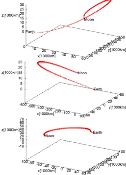
Applying the scheme presented in section 2, we wrote simple C++ program. In every step the algorithm chooses one point on the trajectory, change it and accept the mutation if it leads to the smaller value of the distance d (3). In our simulations we constrained the numbers of points between initial and final time to 200, restricted the maximal mutation value in one step to less than 10−4 _{Earth-Moon distance, and as a} starting and final position of the spacecraft choose respectively the point at 6500 km from Earth center and 2000 km from Moon center. After 8

10

≈ _{iterations from the} random trajectories we obtained the solution which differ from the real one by 6

10

[image:4.595.243.501.74.433.2]

Figure 1. Trajectory to the moon in 7, 14, 21 days.

4. Summary

We presented simple evolutionary algorithm with one trajectory at any given time and mutation as a selection mechanism. By changing the trajectory so as to make equal accelerations and forces, we were able to find a true trajectory which satisfies the Newton’s second law. Trying this scheme for longer times could lead us to find interesting trajectories, for example, with small initial velocity (small rocket fuel consumption).

The general method presented in this article can be used to obtain solution to any physical problem described by mathematical equation. In particular, apart of astrody- namical problems similar to the one presented here, it can be useful in finding the solution of the internal structure of the stars (the values of the observable parameters both at the center and at the surface are given), in statistical mechanics problems like Ising model to obtain phase transition, in fluid dynamics problems where no-slip condition fixes the velocity on the boundaries or heat transfer problems.

References

Aus-tralian Journal of Biological Sciences 10, 484-491. http://dx.doi.org/10.1071/BI9570484 [2] Koza (1992) Genetic Programming. MIT.

[3] Lei, H.L., Xu, B. and Sun, Y.S. (2013) Earth-Moon Low Energy Trajectory Optimization in the Real System. Advances in Space Research, 51, 917-929.

http://dx.doi.org/10.1016/j.asr.2012.10.011

[4] Bate, R.R., Mueller, D.D. and White, J.E. (1971) Fundamentals of Astrodynamics. Dover Publications, New York.

[5] Belbruno, E. (2004) Capture Dynamics and Chaotic Motions in Celestial Mechanics. Prin-ceton University Press, PrinPrin-ceton.

Submit or recommend next manuscript to SCIRP and we will provide best service for you:

Accepting pre-submission inquiries through Email, Facebook, LinkedIn, Twitter, etc. A wide selection of journals (inclusive of 9 subjects, more than 200 journals)

Providing 24-hour high-quality service User-friendly online submission system Fair and swift peer-review system

Efficient typesetting and proofreading procedure

Display of the result of downloads and visits, as well as the number of cited articles Maximum dissemination of your research work