Munich Personal RePEc Archive
A predictive multi-agent approach to
model systems with linear rational
expectations
Mostafavi, Moeen and Fatehi, Ali-Reza and Shakouri G.,
Hamed and Von zur Muehlen, Peter
K.N. Toosi university of technology
8 January 2011
Online at
https://mpra.ub.uni-muenchen.de/35351/
1 Corresponding Author: APAC Research Group, Faculty of Electrical & Computer Engineering, K.N.Toosi University
of Technology,Tehran, Iran, [email protected]
2 APAC Research Group, Faculty of Electrical & Computer Engineering, K.N.Toosi University of Technology,Tehran,
Iran, [email protected]
3 Industrial Engineering Department, University of Tehran, Tehran, Iran,hshakouri@ut.ac.ir
4 Federal Reserve Board, retired, [email protected] Abstract: Expectation formation plays a principal role in economic systems. We examine and revise the standard rational expectations (RE) model, generally taken as the best paradigm for expectations modelling, and suggest a new method to model rational expectations. Conventional conditions that assert the stability and uniqueness of popular solution methods are shown to be insufficient. The agent-based new modelling approach suggested in this paper will be shown to lead to uniquely stable solutions.
Keywords: Rational expectation, Predictive control, Economics dynamic
1
Introduction
Lots of economists believe that the main differences between natural systems and social systems are the forward-looking decisions in social systems. The use of expectations in economic systems goes back to the writings of Greek philosopher Thales of Miletus. Systematic use of expectations in economic modelling began at the beginning of the 19-th century [1]. A modern formal revival of the role of expectations in economics is by Muth [2], who introduced the concept of rational expectations (RE), now widely accepted as a main driving force of expectation formation in contemporary economics.
The main idea in rational expectations is that predictions, always based on currently available information, made by decision making units in an economy, are not systematically wrong in that all errors are random. Because such predictions must, in equilibrium, be consistent with the model describing agents’ behaviour, a better term for rational expectations is “model consistent” expectations. Economists have mostly settled on studying linear versions of dynamic RE models with special applications to the analysis of monetary policy. Because
of the requirement that, in equilibrium, expectations must be consistent with a given model’s predictions and that the solution of the model be uniquely stable, economists have developed a set of what are called “determinacy” conditions necessary for uniquely stable solutions of linear dynamic RE models.
Determinacy conditions were originally derived in 1980 by Blanchard and Kahn (BK) [3] and have since then been widely used by other economists [4-7]. More recently, Sims[8] developed an alternative and more generalized solution technique that is now also widely used in the literature.
However, recently we [9] reported a weakness in the BK determinacy condition, a weakness also observed by Cho and McCallum [10] and Sims [11]. Using some simple contradictory examples, we demonstrated the nature of this weakness and underlying reasons [9].
Since problems with solving RE models are not limited to the BK approach, it is useful to take a fresh look at how to think of and solve dynamic RE systems.
In this paper, we propose a new framework for modelling RE systems, one that is based on predictive control and agent-based modelling. We will show that this framework is consistent Muth’s [2] original conception of rational expectations.
The paper is organized as follows. The following section briefly reviews classical RE models and shows their main practical weaknesses. The next section introduces new tools to model RE systems. We demonstrate the conclusions from our analysis via simulations. The last section gives a summary.
2
Classical RE models
A predictive multi-agent approach to model systems with linear rational expectations
2 to be the best possible estimates. However, as we point out, in classical RE models, certain weaknesses cause some mathematical inconsistencies.
In classical dynamic RE models, one distinguishes between predetermined and non-predetermined variables (also known as jump variables). Predetermined variables have the same structure as state variables in control engineering; but non-predetermined variables are the best estimates of future values of some variables. Based on current information, non-predetermined variables should be replaced by equations of other variables. This procedure is known as the solution method of RE models. To take a closer look, we examine the approach advocated by Blanchard and Kahn[3]
2.1
Summary of BK approach
BK considered the following canonical model [3]:
1 1 X X t t A Z t P P
t t t
γ + = + + (1)
where X0 is given initial state and
Xt: ‘predetermined variables’ (determined in t-1 or earlier)
Pt: ‘jump variables’ (choice variables determined in t)
Zt: exogenous (random) variables | Zt | ≤ M < ∞ tPt+1: expected value of Pt+1at time t:
E(P | )
1 t 1
P
t t+ = + Ωt (2)
where E( ). is the mathematical expectation operator;
( )t
Ω
is the information set at t;Ω
( )t⊇ Ω
(t−1);Ω
( )t includes at least past and current values of X, P, Z, however the information set may include other exogenous variables than Z. Also, it may include future values of exogenous variables.Let
λ λ
1≤ 2 ≤ ... ≤λ
n be n eigenvalues of A (countingmultiplicities). Let n∗ be the number of eigenvalues larger than one, then:
PROPOSITION 1: If n∗=dim P
( )
t then there exists aunique solution.
PROPOSITION 2: If n∗>dim P
( )
t then there is nononexplosive solution.
PROPOSITION 3: If n∗<dim P
( )
t then there is aninfinite number of solutions.
2.2
A practical example
Classical RE models are usually written at an aggregative level, and the stability and robustness of the closed-loop systems are analyzed.
For the example, we take the following model, which is called the canonical New Keynesian model. It is a simplified version of the models which are used by central banks, * * 1 1 * 1 1 , n
x E x r E r
t t t t t t t
kx E
t t t t
n n
r r
t t r t
σ
β
ρ ε
= + − − Π + −
Π = + Π +
= − +
(3)
where x is the log deviation of output from potential output, Π is the inflation rate,
r
is a short-term interest rate controlled by the central bank, andr
n is the natural interest rate---the rate at which output growth proceeds at capacity, and unemployment is at its natural or long-run equilibrium level.The first equation describes aggregate demand (IS); and the second equation is aggregate supply (AS). The system is closed with a policy rule for
r
t , which is the policy instrument. The following commonly described policy feedback rule closes the model,1
r x r
t =φπΠ +t φx t +φr t− (4) In the economic literature the values of ,
x
φ φπ and
r
φ are selected in a way to minimize a quadratic Loss function involving selected the states in the model. In matrix form, the model is written.
* 1 * 0 1 0 1
E x x
t t t
n
E A r
t t t t
r r t t σ + −
Π = Π +
+ − (5)
where A is given below:
1 1 0 1 k k r
x x x
k A
k k k
x x x x x r x
r
x x x
β σφ σ σφ σ σφ
π π
β βσφ β βσφ σφ
β β
φ βφ σφ φ σφ φ σφ φ σφ σφ φ
π π π π φ
β β βσφ β β βσφ σφ
− − − − − − = − − − − − + + + − − −
In this example the BK determinacy criterion holds if and only if two eigenvalues of A have absolute value greater that unity. However, Cho and McCallum [10] and Mostafavi, et. al. [9] have shown that even if BK’s determinacy condition is satisfied, the system may be unstable.
2.3
The main weaknesses of classical methods
3 simplified examples, some fundamental revision in how one approaches dynamic RE models is required.
2.3.1 Structure
Usually, economic systems have a multiple-input multiple-output (MIMO) structure without a centralized controller. In such systems, different agents activate their own inputs to minimize a loss function and thus differ from classical decentralized controllers because the loss function of these agents can have heterogeneous forms. In economic systems, it is possible that all agents act in unison, and it is possible that some agents act to minimize a state while others act to maximize it; and so there may be competition among them. These agents try to estimate the future behaviour of the system, and based on this estimation, they optimally determine the inputs that under their control.
In economic systems, where different agents calculate individual and often conflicting feedback rules, stability and determinacy at the aggregate level is a function of the diverse behaviour of heterogeneous agents within the system.
The inherent MIMO structure of such models and the presence of multi-agent behaviour are usually ignored in classical (engineering) methods. Interactions, not modelled inputs etc. cause some problems in classical methods.
2.3.2 Expectation formation
Expectation formation plays a main role in dynamic economic models. In classical RE models, the expectation terms are manifest in the dynamics of the aggregative closed-loop system; but for analytical purposes, it is necessary to find their disaggregated origins. At the aggregative level of the system, current states are affected by individual predictions of their future values, the aggregated effect having originated in the decision making structure of each agent. Each economic agent estimates future variables relevant to his or her welfare, based on currently available information and behaves in a way that minimizes a loss function unique to the agent. While the effects of individual forecasts made by agents directly determine the structure of current inputs, it is important to note that these effects influence the system’s structure only indirectly. So if we write the equations of an aggregated closed-loop system based on this construct, the prediction terms will also become apparent in the aggregated dynamic structure.
Notice that the predictive control strategy described here is similar to decision making strategies typical in economic systems. Each decision maker knows the desired reference trajectory for a finite control horizon, and by taking into account the economic characteristics (mental model of the economy) decides which control actions (investment, consumption and etc) to take in order to follow the desired trajectory. Contrary to dynamic programming, decision rules in this framework are by definition discretionary: only the first (of a sequence of planned) control actions are taken at each instant, and the procedure is repeated with re-optimization for the next control decisions in a receding-horizon fashion.
Compared with other classical controllers, model-predictive controllers use more information (the reference trajectory), so that the behaviour of each agent is analogous to a predictive controller.
2.3.3 Functional controllability
In economic systems it is usually required that all the states of a system follow a trajectory, which means that each of the states plays the role of an output; and so the concept of functional controllability is needed.
Consider a MIMO plant with m inputs and l output. In order to control all outputs independently the plant must be functionally controllable [13]. A necessary but not sufficient condition for functionally controllability is
m≥l .
Note the differences between the following cases for a system with 2 agents and 2 states,
I. The system has 3 inputs, and 2 of them are determined by the first agent. If the first agent is able to estimate the behaviour of the second agent the system is functionally controllable from the point of view of the first agent
II. The system has 2 inputs, and only one of them is set by the first agent. In this case, the system is not functionally controllable for the first agent, even if it is able to estimate the behaviour of the second agent. The first agent would be able to minimize its own loss function, but this minimization doesn't mean following a trajectory for the system.
From the above brief discussion we conclude that in a macroeconomic system, if the central bank is able to determine only one input (for example, a short-term interest rate) and it wants to control two different states (for example, the inflation rate and the output gap) independently, this would not be possible, even if it is able to estimate the behaviour of all households and firms. In such cases a combination of different policies should be used.
3
New ideas for modeling
3.1
Structure
As originally emphasized by Muth[2], a proper micro-based description of expectations formation is essential for the logical consistency of an economic model and for its empirical relevance. Unfortunately, a common practice today is to write the equations without regard to the origins of the expectations terms. In his original paper, Muth actually gave an example of how one might go about doing this. This paper is an attempt to resurrect Muth’s original point.
A predictive multi-agent approach to model systems with linear rational expectations
4 on their estimation, has the best trajectory for their own welfare function. Each agent’s estimate is based on past values of other parts of economic system, the past value of its own output, and the known trajectory of future inputs to the whole system.
The expectation of future variables is found in the estimator part, and then it is used in the predictive controller.
Summarising, the output of the predictive controller includes the effect of agents' predictions. Writing the system equations based on an aggregation of each agent’s viewpoint produces equations that look like the equations in a typical dynamic RE model but have a number of
different characteristics that are important to stability and uniqueness of the system.
Actual economic systems are, of course the aggregations of individual decision structures like the one just described. In the economic literature, it has been common not to separate heterogeneous components in a model and not to treat each as a unique system with its characteristic dynamic set of equations. For our purposes, we will find it necessary to focus on the separate behaviours of individual decision makers in order to describe a true dynamic rational equilibrium model.
Such a structure, called multi-agent predictive control, has a common framework in control engineering.
! "
# "
"
A structure for economic systems with rational expectation dynamic
Stability, learnability, performance analysis, and robustness analysis of such systems are widely analyzed in engineering, and they can also be used in economic systems.
We note that in the economic literature, RE models are touted as being endowed with model-based expectations[14]. This description of RE models is consistent with the structure proposed here.
3.2
A simple model
Suppose that the system is described by the following difference equations,
1 1
X AX BU CD
t+ = t+ t+ t+ (6)
with the following matrices:
( )
( )
( ) ( )
1 1 1 1 11 12 11 12 11 12
, , , , ,
1
2 1 2 2 21 22 21 22 21 22
11 12 13
21 22 23
X D U a a c c b b
t t
X D U A C B or B
t X D t U a
b b b
b b
a c c b b
t t b
+
= = = = = = =
+
+
where,
Xt: State variables
Ut: Exogenous variable
Dt: An iid noise
A, B, C: Constant matrices of appropriate size.
Note that U1(t) is a exogenous variable from the view point of the second agent and vice versa.
The best estimation of this system based on current information is,
1
X AX BU
t t+ = t+ t (7)
Finding the expectation for q steps ahead results in
( )
( )
11
q
q q i
X A X A BU
t t q t t i
i
− = + ∑
+ = + − (8)
Since the estimators of prediction terms are minimum state variables, their result will be unique. Each agent tries to minimize its loss function which has the following form,
(
) (
)
1
1
1( ) , ,
n
w
T
w
L X X X X
t =
∑
=β − t t+w − d t+w t t+w − d t+w (9)5 of decision making (controller) to minimize its own Loss function,
, ( ),
1( ) 2 ( )
U f X U t k X
t t d t k
= + + (10)
where f (.) is a function which is found by the minimization procedure. Knowing this structure the system equation is rewritten as,
, ( ),
1 1 2 ( ) 2 2( ) 1
X A X b f X U t k X b U CD
t t t d t k t t
= + + + +
+ + +
(11)
where b1 is the part of B which is related to the first agent and b2 is the part of B which is related to the second agent.
The above equation can be used to describe the system equation from the second agent’s point of view. This equation is in the form of a solutions to the RE system. The main difference between the solution of this model and the traditional solution of RE models is in the modeling of the expectation terms in the loss function of each agent instead of in their dynamic recursions. This means essentially that we have retained the same structure as the typical RE model.
In a special case, if the optimization horizon in the loss function for the first agent is set to be n = 3, the function
f (.) can be found by a routine procedure.
Since estimates of states at time t + d depend on the choice of future input signals, it is necessary to make some assumptions about them. One possibility is to assume that the first agent has some information about input signals which are determined by the second agent, while its own input signal remains constant for the optimization horizon. In other words we assume that
1( ) 1( 2) 1( 3)
U U U
t = t+ = t+ and tU2(t+k) k=1, 2,...
are known.
With the above assumptions, the optimal controller for this agent can be obtained as:
1 1( )
U F G
t = − −
(12)
where F and G are given in the next page.
In this simple structure we assume that the second agent is not using a feedback rule. Although in a real world, most or all agents use feedback rules, we use this simplifying assumption to illustrate the main concept. Replacing the optimal solution for the first agent, the stability of the system can be analysed by the eigenvalues of the following closed-loop transition matrix.
4
A simple example
4.1
Functional controllable system
Suppose that the system structure is in the same form of (6), and that the system matrixes are given by (13) and (14), where N is the simulation horizon. Assume that N = 100. The discount factor is set to be β =0.8. In the simulation we assumed that the behaviour of the second agent is estimated by the first agent with noise, tU2(t+1)=U2(t+1) + nd(t), where nd(t) ~ iid(0,0.01).
To analyse the stability of the system, it is only required that the absolute value of all the eigenvalues of the closed loop state transition matrix be smaller than one. The eigenvalues of open-loop system are
[
1.4071 -0.0071]
. Since the absolute value of one of them is greater than one, the open-loop system is unstable. But since the eigenvalues of the closed-loop system are[
0.8671 -0.2667 , the closed loop system is stable.]
0 10 20 30 40 50 60 70 80 90 100
-3 -2.5 -2 -1.5 -1 -0.5 0 0.5 1 1.5 2
Control effort
[image:6.595.336.504.204.335.2]U11 U12
Figure 1. The exogenous variables which are implied by the first agent when the system is functional controllable
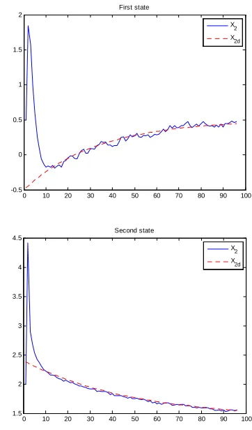
0 10 20 30 40 50 60 70 80 90 100 -0.5
0 0.5 1 1.5 2
First state
X2 X
2d
0 10 20 30 40 50 60 70 80 90 100 1.5
2 2.5 3 3.5 4 4.5
Second state
X2 X
2d
[image:6.595.329.510.376.684.2]A predictive multi-agent approach to model systems with linear rational expectations
6
(
) (
)
(
) (
)
2 2 2 ( )
1 1 1 1 1 1 1 1 1 1 1 1
T T T
F=β A b +Ab +b A b +Ab +b +β Ab +b Ab +b + b b
(
)
(
)
2 ( )
1 1 2 2( ) 2 2( 1) , 2 1 2 2( ) , 1 2 2
2 2( ) 2 2
1 1 1
2 2( 1) 2 2( 2) , 3
T T
A b b A X A b U b U X b A X b U X
t t t d t t t d t
G A X A b U
T t t
A b A b b
Ab U b U X
t t d t
β
β
+ + + + − + + − +
+ + +
= + +
+ + +
+ + −
+ + +
(
)
(
)
1 2 2 2 2
1 1 1 1 1 1
T
T T
A A F Ab b A b A A b A b b A
cl β β
−
= − + + + + + +
(13)
1.3 0.7 1 0
, , , (0,0.05),
1
0.2 0.1 0 1
3 / 0.5 /
(0, 0.01), 2 ,
2 2( ) ( )
2.4 0.6 1 C 1.
2 /
3 2 1.
1. 4
4
A B D iid
t N e t n
D iid U e X
t d t t N
e
= =
−
−
−
= − =
− +
=
∼
∼
(14)
4.2
Nonfunctional controllable system
In the previous section, we assumed that the first agent is able to implement two different exogenous variables, and so the system was functionally controllable for it. Since the system was functionally controllable, the state trajectories were similar to the desired trajectory of the first agent. In the following simulation it is assumed that the first agent is able to implement one exogenous variable only, rendering the system functionally uncontrollable.
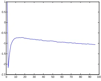
0 10 20 30 40 50 60 70 80 90 100
[image:7.595.128.505.82.574.2]-2.5 -2 -1.5 -1 -0.5 0 0.5 1
Figure 3. The exogenous variable which is implied by the first agent when the system is not functional controllable
From the figures it is clear that the trajectory of the second state is remarkably different from the desired trajectory of the first agent. It should be noted that this response is the optimal solution from the view point of the first agent as it minimizes its loss function.
To be able to compare the functionally controllable system with the second functionally uncontrollable system, the simulations are repeated for N = 1000. The implied loss functions attained the following values: For the functionally controllable system, loss = 118.4436 For the functionally uncontrollable system, loss = 1085.5.
0 10 20 30 40 50 60 70 80 90 100
-1 0 1 2 3 4 5 6
First state
X2 X2d
0 10 20 30 40 50 60 70 80 90 100
0.5 1 1.5 2 2.5 3 3.5 4
Second state
X2 X2d
Figure 4. Tracking of the states in a system which is not functional controllable in the view point of the first agent
5
Conclusion
The insufficiency of BK’s determinacy condition in some instances of dynamic rational expectations models impelled us to seek alternative criteria to ensure stability and uniqueness. To accomplish this goal, we propose a new model structure for RE systems based on heterogeneous agents.
[image:7.595.90.255.423.556.2]7 demonstrate that our approach is both analytically tractable and sufficient for analyzing the stability and performance of dynamic RE models, suggesting a potential of this methodology as a strong tool in the literature.
In this brief report, we use a simple example to show the consistency of this structure with classical RE models. In the real world, most agents can reasonably be assumed to employ some version of predictive control, even though details will likely differ from the examples offered here. Whatever the case is, identification procedures should be added to any proposed system. Furthermore, given the competitive nature of markets in economies, inherent game-theoretic elements need to be addressed regarding decision rules and expectations formation.
Finally, this paper’s focus on stability analysis does not preclude future work to investigate robustly stable structures.
ACKNOWLEDGMENT
The authors would like to acknowledge and extend their heartfelt gratitude to Prof. Caro Lucas who helped us in this project but passed away.