The US monetary performance prior to the 2008 crisis

The US monetary performance prior to

the 2008 crisis

Li, Kui-Wai

2012

Online at

https://mpra.ub.uni-muenchen.de/41036/

Applied Economics, 45 (24), 2013: 3449-3460

The U.S. Monetary Performance Prior to the 2008 Crisis

Kui-Wai Li

Abstract

This article uses a structural VAR approach to study the different shocks to the monetary performance in the two decades of the U.S. economy prior to the 2008 financial crisis. By using the Federal Fund Rate as a measure of change in monetary policy, the study shows that interest rate expectation is informative about the future movement of Federal Fund Rate and the anticipated monetary policy should be one of the crucial reasons in causing monetary and financial deterioration in the U.S. economy. The article discusses a possible conjecture of a low interest rate trap when a persistent and prolonged low interest rate regime led to financial instability.

JEL classification: C32; E52; O51.

Keywords: Monetary shocks; Interest rate; Financial crisis.

____

Kui-Wai Li, Department of Economics and Finance, City University of Hong Kong. Tel.: 852-3442 8805; fax: 852-3442 0195; E-mail address: [email protected]

I Introduction

Since banks and hedge funds have invested heavily in subprime mortgage backed

securities, few have predicted that the U.S. subprime mortgage industry could lead to a

worldwide credit crunch when the Fed takeover the two mortgage-based security companies and

the closure of Lehman Brothers. Efforts have been made to rescue the subsequent economic

collapses (Financial Services Authority, 2009; French et al., 2010; IMF, 2009). The 2008 crisis

has raised the relevance of monetary fundamentals (Taylor and Williams, 2009; Taylor, 2009).

Schwartz (2009) explained that expansive monetary policy, flawed financial innovations and

collapse of trading contributed to the 2008 financial crisis.

Studies on the U.S. monetary economy have identified five monetary features under Alan

Greenspan’s chairmanship (7/1985 to 8/2005) of the U.S. Federal Reserve. The practice of a direction-known interest-rate smoothing policy showed a stepwise interest rate trend. It has the

advantage of financial stability and certainty, but since it could be anticipated, the Fed could not

respond swiftly to shocks, and the resulting inflation variability might have introduced instability

and volatility (Bullard and Mitra, 2007; Caplin and Leahy, 1996; Goodhart, 1996; Cecchetti,

1996). The Fed practiced inflation-targeting and an open acknowledgement for low long-run

inflation (Mankiw, 2002; Blinder and Reis, 2005; Goodfriend, 2005; Bernanke and Mishkin,

1997). Monetary discretions made without pre-commitment to future course of action had

resulted in uncertainty and time-inconsistency (Kydland and Prescott, 1977; Fischer, 1990; Barro

and Gordon, 1983; Bryant et al., 1993, McCallum, 1988). The adoption of the Taylor rulecalled

for changes in the Federal Fund Rate in response to changes in the price level, although there

were periods of deviation (Taylor, 1993; Yellen, 2004; Mehra and Minton, 2007; Blinder and

Reis, 2005; Woodford, 2001). The personalization of monetary policy (Greenspan put) has led to

a belief that stock markets would be saved when it went downbut would not intervene to stop it

from rising (Miller et al., 2002).

This article examines the monetary fundamentals of the U.S. economy in the two decades

leading up to the 2008 financial crisis. The monthly U.S. data are obtained from the DataStream

and International Financial Statistics (IFS) for the sample period between 1989.1 and 2008.7

prior to financial crisis in September. A structural VAR approach is used to study monetary

shocks in the two decades of the U.S. economy. Section II examines the monetary performance

Section III and IV present the empirical methodology and the empirical findings, respectively.

Section V concludes.

II Monetary Performance and Conjecture

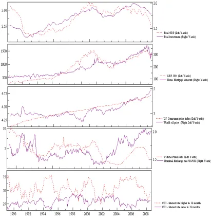
Figure 1 shows the performance of ten U.S. variables prior to the 2008 financial crisis.

Real GDP and real investment show the level of economic activities. The monthly real GDP and

real investment data are constructed from quarterly data by the state space approach with the

monthly industrial production data serving as the interpolator variable, assuming that the

interpolation is describable as an AR(1) process. The U.S. recession in the mid-1980s has

resulted in prolonged economic weakness with a fall in real GDP and real investment until 1992.

The nominal economic variables include S&P500 and home mortgages; they both were

bullish and increased continuously to a historical high level until early 2008. For example, the

Nasdaq Composite Index lost half of its points between March and December, 2000, and

declined further after the 2001 terrorist attack. In the real estate market, the 1995 Community

Reinvestment Act was reformed, while the 1997 Taxpayer Relief Act exempted tax from profits

made from sales of residences up to US$0.5 million for married couples. Home ownership

peaked in 2004, but signs on the end of the housing boom appeared in 2005. In early 2007, the

problem of subprime mortgage surfaced with Bear Stern closed one of its funds.

While the core Consumer Price Index (CPI) excludes the price influence of food and

energy, the drastic increase in the world price of oil (OPW) has affected the U.S. economy. The

inclusion of OPW ensures that the estimation model will not suffer from the ‘price puzzle’ problem (Sims, 1992, Sims et al., 1996; Christiano et al., 1996). The core CPI has increased

continuously, and followed closely the OPW trend. The OPW has shown a steady trend in the

1990s, but has increased rapidly since 1999.

The fourth chart shows the Federal Fund Rate (FFR) and the nominal exchange rate (EX)

of the U.S. dollar against the British pound is used as the unit of measure in capital flows. A

sustained upward movement in EX since 2002 showed that there was capital outflow due

probably to the historical low level of FFR. The two indicators of consumer confidence index in

12-month interest rate higher (RH) and 12-month interest rate same (RS) are used as measures

on consumer behavior and the dynamic response of the economy to shocks in interest rate

remained high at different time periods, and has fluctuated more than the latter. The interest rate

expectation of consumers is highly volatile at around 35% to 75% from 1989 to 1993, when

investors did not seem to have definite expectation on the future interest rate.

Figure 1 Log U.S. Variables

The FFR trend shows two prolonged low interest rate periods (1993-1995 and

2002-2004), with a clear downward movement in 1989-1994 when it was lowered from 6% to 1.75%

in 2001. Economic recovery that began in 1992 suggested that the low interest rate policy could

steps to lower interest rates. Changes in interest rate expectations often occurred in months ahead

of the FFR movement, implying a full anticipation of the monetary policy by investors. Starting

from 2004, the adjustment on the FFR was not effective in controlling the overheated real estate

market. The increase in the FFR from 1% to 1.25% on June 30, 2004, brought a two-year upward

trend. This could be due to the full anticipation by investors, as high interest rate expectations

remained steady between 2004 and 2006, though one could interpret that the low FFR between

2002 and 2004 have stimulated investment, and continued to impact output till 2006.

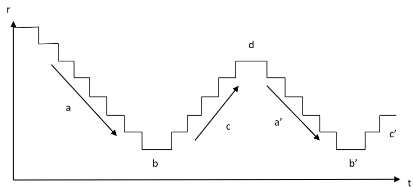
Once investors’ prediction on monetary policy became more accurate over time, interest rate movements might become ineffective in stabilizing business cycles and promoting long-term

growth. The monetary conjecture in Figure 2 stylizes the steps and responses in Greenspan’s interest-rate policy. When the interest rate fell (arrow “a”) and if investors could fully anticipate the next round of interest rate movements, investors would have waited till the interest rate has

fallen to its lowest possible level. The initial fall in the interest rate might not lead to much

economic adjustment (Lucas, 1981; Sargent and Wallace, 1975; Modigliani, 1977; Barro, 1976).

As such, policymakers might think that a further drop in interest rates was needed in order to

stimulate investment. It was probable that when the interest rate had reached a very low level,

“b”, investors would then borrow extensively. The extremely low interest rate now would encourage unproductive, low-return and speculative bubble-prone varieties.

The rapid increase in investment at the low interest rate could produce overheating that

called for policy reversal (arrow “c”). The initial reversal in interest rates could even lead to a rise in investment as investors expected higher future borrowing cost. The rise in interest rate

would soon lower economic activities. Those who have borrowed at the lowest interest rate at “b” would now face a repayment problem. By the time the interest rate reached a high level, “d”, economic slowdown emerged and the authority would then have to revise the interest rate

downward, producing another round of stepwise downward movement in interest rate policy

(arrow a’, b’ and c’).

When investors could fully anticipate the interest rate movements, fragile investors would

wait until interest rate reached the lowest possible level. For example, home ownership was

encouraged during the second term of the Clinton administration. As property prices rise the

demand for property also rises as home buyers now feared that property prices would soon rise

expected rising property price. The monetary conjecture in Figure 2 shows that the economy

could have been “trapped” at the lowest interest rate levels at points b and b’, as investors have got used to the low interest rate and monetary authority found it difficult to maintain a higher

level of interest rate. A prolonged low interest rate regime could have encouraged financial and

property speculations that cumulated to form the roots of a financial bubble. A stepwise interest

rate smoothing policy could eventually produce an unsustainable and cyclical form of monetary

policy that helped more to fuel financial instability than to build up sustainable economic

capacity. The economy was effectively addicted to a low interest rate regime, making financial

resources cheap and promoting low-productivity. While the Fed attempted to manage the

business cycle, the interest rate policy could have led to a trade-off in sustainable long-run

growth.

Figure 2 Conjecture of a Low Interest Rate Trap

III Model Identification

The “low interest rate trap” can be studied using U.S. data to show if interest rate followed a stepwise movement and investors anticipated fully its movement. A structural vector

autoregressive (SVAR) model (Sims and Zha, 2006; Kim and Roubini, 2000) is used to

incorporate the interest rate expectation of investors to show that monetary policy could become

ineffective and/or would promote speculation when it is fully anticipated.

The following SVAR system expresses the contemporaneous interactions between the

variables in structural form:

r

t a

b

c d

a’

b’

0

( ) _{t t}

B L Y  e , (1)

where B(L) is a n x n matrix polynomial in the lag operator, L; Yt is a n x 1 vector of variables,

and et is a n x 1 vector structural disturbances which is identical independent normal with var (et)

= . The is a diagonal matrix and the diagonal elements are the variances of structural

disturbances such that each structural disturbance can be assigned explicitly to particular

equations. Let B0 be the contemporaneous coefficient matrix on L0 in the structural form, and

let 0_{( )}

B L _{be the coefficient matrix in} B(L) without contemporaneous coefficient B0. The matrix

polynomial in the lag operator, L, is expressed as:

0 0

( ) ( )

B L B B L . (2)

Consider the reduced form VAR equation:

0 ( )

t t t

Y  A L Y u _{, (3)}

where A(L) is a matrix polynomial in lag operator, L, and μt is a vector of reduced-form

disturbances with no structural interpretation. Multiply 1 0

B to the structural form equation:

1 1 1

0 0 0 ( ) 1 0 0 ( ) 1

t t t t t

Y B B B L Y _ B e  A L Y_ u . (4)

The parameters of reduced form VAR equation are related to the parameters of the SVAR

equation:

1 0 0

( ) ( )

A L B B L . (5)

The reduced form residuals are related to the structural disturbances:

1 0

t t

u B e _{, (6)}

and its covariance matrix is:

'

' 1 1

0 0

( _{t t})

E u u   BB _{. (7)}

The reduced form residuals become the linear combinations of the structural disturbances.

Equation (7) suggests that the covariance matrix of the reduced form residuals is not diagonal,

and the right hand side of the equation has n (n 1) free parameters to be estimated. Since 

contains n(n1) / 2 parameters, the parameters in the SVAR equation cannot be identified

without restriction. To achieve identification, n (n 1) / 2 _{restrictions are needed. By}

normalizing the diagonal elements in B0 to unity, the identification requires at least

( 1) / 2

policy and interest rate expectation shocks and to estimate their effect on output variables. A

number of zero (exclusion) restrictions are imposed on the contemporaneous structural

parameters, B0 , in Equation (6). The following equations show the identification restrictions:

, ,

, ₂₁ ,

, _{31 32} ,

, 41 46 ,

51 52 53 54

, ,

61 62 63 64 65

, ,

1 0 0 0 0 0

1 0 0 0 0

0

1 0 0

0 0 1 0

0 1

1

OPW t OPW t

Y t Y t

CPI t CPI t

FFR t FFR t

RH t RH t

EX t EX t

e u

e _b u

e _{b b} u

e b b u

b b b b

e u

b b b b b

e u   _{ }    _{ }    _{ }    _{ }    _{ }    _{ }    _{ }    _{ }      _{ }     

.

The terms on the LHS of Equation (8) show the six sub-equations in the structural model

represent the unobserved structural shocks, while ui,t are the observed residuals obtained from the

reduced form of VAR analysis. As oil is imported to the U.S. economy, the first sub-equation

assumes that OPW is exogenous to the U.S. economy. The second output sub-equation shows

that output responds mainly to OPW shocks. However, it also assumed that CPI, FFR, RH and

EX impact on the lag values of output. In order to incorporate the influence of real investment,

S&P500 and home mortgages, Equation (8) will be tested in three alternative models with real

investment, S&P500 and home mortgages subsequently replacing output in the second

sub-equation. The output, S&P500 and real investment are considered as the dependent variable in

each model, and their fluctuation depended on OPW, CPI and so on.

The third sub-equation shows the response of CPI with respect only to output and OPW

shocks. In the S&P500 model identification in the second sub-equation, it is assumed that the

movement of the S&P500 index return would not result in contemporaneous price level

fluctuation. The coefficient estimate of b32 would become zero. We further assume that the

S&P500 index return will contemporaneously respond to the FFR and EX shocks (Ehrmann and

Fratzcher, 2004). A negative relationship between exchange rate and stock return would produce

a non-zero coefficient estimate for b24 and b26(Solnik, 1987; Wong and Li, 2010).

The fourth sub-equation is a monetary policy feedback equation, as the Fed adjusted FFR

in response to the OPW and EX. The monetary policy function does not response to output and

CPI contemporaneously as it experienced information delays (Sims and Zha, 2006). But

fifth sub-equation represents the interest rate expectation function which is assumed to respond

contemporaneously to all variables except EX, as short term EX fluctuation would not affect

investors’ expectation on interest rate. Lastly, the exchange rate equation is assumed to be related to all variables in the system of equations.

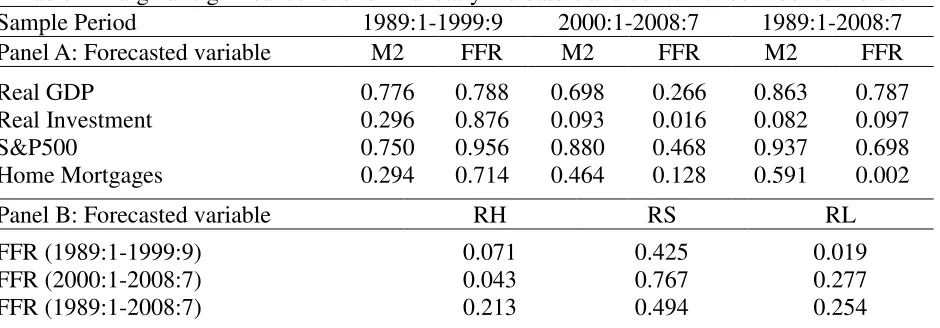
Table 1 Marginal significance level of monetary indicators and consumer confidence indices Sample Period 1989:1-1999:9 2000:1-2008:7 1989:1-2008:7 Panel A: Forecasted variable M2 FFR M2 FFR M2 FFR

Real GDP Real Investment S&P500 Home Mortgages 0.776 0.296 0.750 0.294 0.788 0.876 0.956 0.714 0.698 0.093 0.880 0.464 0.266 0.016 0.468 0.128 0.863 0.082 0.937 0.591 0.787 0.097 0.698 0.002

Panel B: Forecasted variable RH RS RL FFR (1989:1-1999:9) FFR (2000:1-2008:7) FFR (1989:1-2008:7) 0.071 0.043 0.213 0.425 0.767 0.494 0.019 0.277 0.254 Notes: For each row of the forecasted variable, the estimated value represents the marginal significance level for omitting six lags of M2 or FFR from an unrestricted OLS equation which included a constant, trend, six lags of price level, and six lags of the forecasted variable. RH, (RS) and [RL] correspond to consumer confidence index – interest rate higher, (same) and [lower] in 12 months. The estimated values in Panel B represent the marginal significance level for omitting six lags of RH, RS or RL from an unrestricted OLS equation that included a constant, trend, and six lags of the forecasted variable.

The two sub-sample periods (1989:1-1999:9 and 2000:1-2008:7) used in the analysis of

the September 2008 crisis reflected the dotcom bubble, change of U.S. leadership in 2000 and

2001 terrorist attack. Data are expressed in logarithm and first-difference-stationary verified by

the Augmented Dickey-Fuller (ADF) test. The Granger-causality test is conducted to select

whether M2 or FFR is appropriate for our analysis (Bernanke and Blinder, 1992; Sims and Zha,

1994). Table 1 Panel A shows the marginal significance level that the lags of either M2 or FFR

should be excluded from the equation. Given that smaller estimates are preferred, FFR is

superior to M2 in the second sub-sample period but not in the first sub-sample period. For the

whole sample period, FFR outperformed M2 as a preferred variable in forecasting other variables.

In forecasting the FFR, Panel B reports the marginal significance levels of consumer confidence

index on higher (RH), same (RS) or lower (RL) interest rate in 12 months. Among the three

period, as seen from the smaller value of the estimates. The level of statistical significance for

RH in the first and second sub-sample periods is 10 percent and 5 percent, respectively. RH has

shown a higher predictive power in the second sub-sample period than in the first sub-sample

period. FFR is used as a monetary policy indicator while RH is the interest rate expectation

indicator in the estimation.

IV Empirical Results

We examine from Equation (8) the influence of FFR and RH on output, investment,

S&P500 and home mortgages over the two sub-sample periods. The number of lag length in each

model is based on the Akaike information criterion. The constant and trend variables are included.

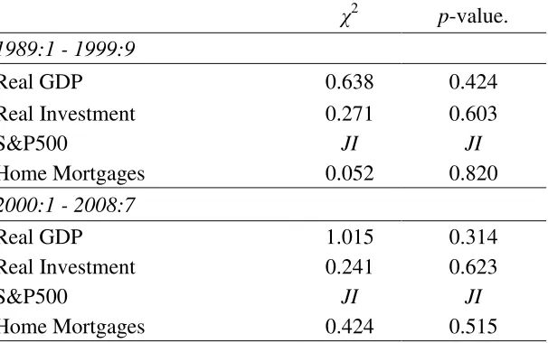
Table 2 reports the Likelihood Ratio Test results for over-identification restriction, and that

output, investment and home mortgages are over-identified, while S&P500 is just-identified. The

p-value corresponds to the hypothesis test of the single over-identification restriction, and a

coefficient greater than 0.05 indicates that the particular model cannot be rejected at the 5

percent significance level. Despite the over-identification in some variables that poses unknown

problems, one can still estimate the matrix presented in Equation (8).

Table 2: Likelihood Ratio Test for Over-Identification

χ2

p-value.

1989:1 - 1999:9

Real GDP 0.638 0.424

Real Investment 0.271 0.603

S&P500 JI JI

Home Mortgages 0.052 0.820 2000:1 - 2008:7

Real GDP 1.015 0.314

Real Investment 0.241 0.623

S&P500 JI JI

Table 3: Contemporaneous Coefficients in Structural Models

Real GDP Real Investment S&P 500 Home Mortgage Amount

1989-1999 2000-2008 1989-1999 2000-2008 1989-1999 2000-2008 1989-1999 2000-2008

b21 0.000 0.000 0.011 0.010 0.023 -0.080 0.218 0.020

(0.000) (0.000) (0.007) (0.008) (0.113) (0.231) (0.061) (0.049)

b24 - - - - 0.115 -0.510 - -

- - - - (0.379) (1.593) - -

b26 - - - - 0.582 -1.576 - -

- - - - (1.267) (5.836) - -

b31 -0.009 -0.021 -0.009 -0.021 -0.009 -0.021 -0.008 -0.021

(0.002) (0.003) (0.002) (0.003) (0.002) (0.003) (0.002) (0.003)

b32 0.209 -0.221 0.045 0.067 - - 0.003 -0.008

(0.629) (1.169) (0.023) (0.033) - - (0.003) (0.005)

b41 -0.050 0.230 -0.298 -0.049 -0.090 -0.213 -0.149 -0.169

(0.432) (0.243) (0.205) (0.126) (0.267) (0.831) (0.106) (0.374)

b46 12.423 6.382 4.872 0.641 -2.596 -5.522 -0.328 -7.166

(42.915) (3.619) (3.621) (1.324) (6.742) (22.122) (1.585) (9.560)

b51 -0.120 0.000 -0.333 -0.066 -0.067 -0.010 -0.197 -0.095

(0.349) (0.124) (0.188) (0.131) (0.374) (0.213) (0.159) (0.121)

b52 13.469 66.201 -5.850 -4.807 1.077 -1.005 0.136 0.278

(332.256) (50.998) (2.579) (1.300) (2.573) (2.633) (0.198) (0.202)

b53 -17.748 -4.672 -8.753 -8.510 -6.627 -4.885 -2.529 -4.699

(58.780) (3.738) (7.501) (3.822) (8.184) (5.283) (6.768) (3.492)

b54 1.781 0.048 0.549 0.044 -0.555 -0.150 -0.200 -0.150

(12.281) (0.162) (0.529) (0.089) (1.107) (0.672) (0.224) (0.279)

b61 -0.165 -0.001 0.017 0.004 -0.150 -0.167 -0.069 0.109

(0.534) (0.047) (0.066) (0.034) (0.233) (1.130) (0.045) (0.135)

b62 81.327 88.150 1.338 1.249 -0.304 2.918 -0.078 0.232

(183.497) (27.467) (0.838) (0.362) (1.245) (15.105) (0.046) (0.369)

b63 -3.991 1.424 -0.031 1.829 1.053 3.773 0.602 -2.177

(38.640) (1.434) (2.985) (1.016) (2.241) (15.125) (1.554) (4.252)

b64 -0.907 -0.363 -0.456 -0.061 0.225 0.734 0.036 0.579

(1.328) (0.123) (0.258) (0.068) (0.491) (4.127) (0.162) (0.963)

b65 0.920 0.064 0.199 -0.021 0.163 0.236 0.061 0.074

(3.446) (0.062) (0.186) (0.026) (0.378) (2.584) (0.021) (0.264)

Table 4 Variance Decomposition of Real GDP, Real Investment, S&P 500 and Home Mortgages

Shock 1 (eOPW) Shock 3 (eCPI) Shock 4 (eFFR) Shock 5 (eRH) Shock 6 (eEX)

1989-99 2000-08 1989-99 2000-08 1989-99 2000-08 1989-99 2000-08 1989-99 2000-08

Variance decomposition of real GDP

1 1.4 0.03 0 0 0 0 0 0 0 0

2 1.46 0.94 0.03 1.2 0.05 1.26 0.01 0.22 0.98 0.8

3 1.81 2.26 0.09 2.09 0.06 3.11 0.03 1.36 1.26 0.68

5 2.63 3.06 4.97 3.38 0.05 4.96 0.41 6.64 3.14 1.04

8 3.52 3.81 10.75 8.92 2.82 6.65 0.89 8.56 3.2 1.45

12 5.62 5.42 10.49 9.73 3.15 7.9 0.98 8.64 3.34 2.03

Variance decomposition of real investment

1 1.92 1.39 0 0 0 0 0 0 0 0

2 3.27 3.87 2.88 3.13 0.28 0.62 0.11 1.33 0.16 0.45

3 4.68 3.32 2.9 7.9 1.22 0.42 0.76 4.24 0.28 0.43

5 6.51 3 2.78 12.57 2.37 1.89 1.65 8.77 0.31 6.26

8 6.17 6.88 2.83 10.81 2.34 8.3 1.77 7.87 0.38 6.99

12 6.25 6.67 2.84 9.58 2.41 8.55 1.8 12.82 0.38 6.43

Variance decomposition of S&P 500

1 1.85 0.39 0.15 0.66 1.01 2.31 5.48 1.98 20.32 64.14

2 5.9 6.09 0.88 1.81 1.41 3.08 7.42 2.12 18.53 58.86

3 7.25 6.64 0.98 2.25 1.41 6.01 7.31 3.7 18.21 54.07

5 7.23 7.37 1.07 2.62 1.41 5.89 7.28 3.91 18.18 53.44

8 7.24 7.35 1.08 2.64 1.41 6 7.28 3.97 18.18 53.31

12 7.24 7.35 1.08 2.65 1.41 6 7.28 3.97 18.18 53.3

Variance decomposition of Home Mortgages

1 8.94 0.16 0 0 0 0 0 0 0 0

2 9.81 0.14 0.03 1.06 0.36 0.93 0.01 3.97 0.02 1.83

3 9.82 1.08 0.05 1.09 1.64 1.72 2.74 7.34 0.02 4.13

5 9.86 8.73 0.22 1.66 1.87 2.47 3 11.76 0.15 8.53

8 9.86 7.62 0.24 11.14 1.97 6.36 3.02 10.49 0.16 11.58

12 9.86 7.22 0.24 11.32 1.97 7.62 3.02 11.35 0.16 16.52

Note: Shock 2 (own shock) is excluded.

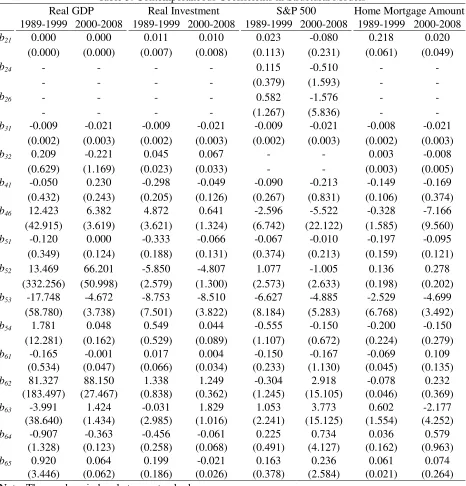
Table 3 shows the contemporaneous coefficients in the four structural models. The

expected relationship of a negative contemporaneous coefficient between S&P500 and FFR (b24

= -0.510) and between S&P500 and EX (b26 = -1.576) appeared only in the second sub-sample

period. For the coefficients estimates of the monetary policy feedback equation (the fourth

S&P500 and home mortgages models. The Fed did increase interest rate when faced with an

unexpected increase in both OPW and unexpected EX depreciation in the second sub-sample

period. However, instead of a positive relationship, the unexpected estimated values of b51 and

b53 are negatively related to the interest rate expectation, implying that investors expected higher

interest rate when negative OPW or CPI shocks occurred.

Importance of interest rate expectation on real output and alternative variables

The forecast error variance decomposition (FEVD) method is used to investigate the

contribution of each structural shock in affecting other variables. Table 4 shows that the

contribution of FFR (shock 4) and interest rate expectation (shock 5) have significantly increased

in the second sub-sample period in most cases, suggesting that their impact on the variance of the

real GDP, real investment, and home mortgages in the second sub-sample period was larger than

in the first sub-sample period. Hence, when interest rate was low, the FFR and interest rate

expectation become more important. In the case of the variance decomposition of real investment,

the contribution by CPI (shock 3) and interest rate expectation (shock 5) have outperformed

other variables in the second sub-sample period, implying that CPI and interest rate expectation

were more important than other variables. The outperformance can be seen from the larger

values shown in Table 4. The significance of CPI was probably due to the high OPW in the

second sub-sample period. The significance of interest rate expectation suggested that investors

could have anticipated interest rate movement, and acted on their investment decisions

accordingly.

For the variance decomposition of S&P500, the contribution of EX (shock 6) is

significantly higher than the others, suggesting that the U.S. stock market is heavily influenced

by EX. The FEVD analysis demonstrates that the higher contribution on the errors in forecasting

real GDP, real investment and home mortgage is due to the variability in the shocks of FFR

(shock 4) and interest rate expectation (shock 5) in the second sub-sample period, as seen from

the larger values of the estimated coefficients for shocks 4 and 5 when compared to other shocks.

Effectiveness of monetary policy and the impact of interest rate expectation (RH) on output

If a monetary policy failed to generate an impact expected by the policy makers, one

possible reason could probably be due to investors’ expectation on interest rate. For example, if investors expected the borrowing cost to remain the same, they might not borrow in the initial

stage of a falling interest rate, but should they subsequently anticipate a reversal in interest rate,

investor might then choose to borrow before rise in borrowing cost. Investors might show an

abrupt change in their expectation on interest rate movement. The impulse response functions

can provide a quantitative measure of the dynamic effects of investors’ interest rate expectation changes. For the purpose of comparison, we consider an interest rate expectation shock with a

structural one standard deviation positive innovation over a horizon of 12 months.

Figure 3 illustrates the impulse response functions of real GDP, real investment, S&P500

and home mortgages to a positive interest rate expectation shock. This enables us to examine the

long term impact of interest rate expectation had on GDP, investment, S&P500 and home

mortgages. A positive interest rate expectation shock represented an increase in the percentage of

the investors who expected the interest rate to rise in the next 12 months. Panel A and Panel B in

Figure 3 represent the two sub-sample periods, and the upper and lower dashed lines plotted in

each chart show the two-standard-error bands generated by Monte Carlo techniques. In response

to an interest rate expectation shock, real GDP responded sharply in the second sub-sample

period, while S&P500 responded inversely in both periods. One can conclude that a positive

interest rate expectation shock did encourage speculation in the second sub-sample period.

To consider the predictability of investors on the interest rate movement, we examine the

dynamic response of interest rate expectation to a positive monetary policy shock, meaning that

when investors expected a high interest rate, the Fed would increase the interest rate. Figure 4

shows the estimated impulse response functions of interest rate expectation to a monetary policy

shock using the real GDP equation. Figure 4 Panel A shows that a positive monetary policy

shock (a rise in interest rate) has generated a negative effect on interest rate expectation until the

fourth month and then moved around the zero line after the sixth month. On the contrary, a

positive reaction is shown in Panel B, and the highest impact came in the fourth month. This

suggested that the positive impact on the interest rate expectation lasted for at least 4 months.

One would conclude that the interest rate smoothing policy was well anticipated by investors in

Note: Panel A=1989-1999, Panel B=2000-2008.

Figure 4 Response of Interest Rate Expectation (RH) to Monetary Policy (FFR) Shock

Dynamic responses to monetary policy (FFR) shocks

It is equally important to illustrate the dynamic responses of economic variables to

monetary policy shocks. The reason for the contractionary monetary policy was to control

inflation and cool the overheated economy. The response functions of the price level and

exchange rate as implied by the real GDP are shown in Figure 5. This shows what response CPI

and exchange rate would have when there was an increase in interest rate. In response to a

contractionary monetary policy shock, Figure 5 Panel A shows that the price level increased

slightly in the first sub-sample period, but dropped below zero after the fifth month, confirming

that contractionary monetary shock did not generate a persistent rise in price level. In Figure 5

Panel B, the price level dropped after the second month, which is consistent with expectation. It

is obviously that a contractionary monetary policy shock produced a larger effect in lowering

inflation rate in the second sub-sample period. In the case of the exchange rate, no significant

effect can be found between the two sub-sample periods.

We next examine the dynamic responses of real GDP, real investment, S&P500 and home

mortgages to a contractionary monetary policy shock (rise in interest rate) (Figure 6). The results

of Figure 6 Panel A are expected and consistent. A contractionary monetary policy shock is

expected to result in a decrease in real GDP, real investment, S&P500 and home mortgages. In

particular, it has a significant negative effect on real investment, S&P500 and home mortgages in

the short run. In Figure 6 Panel B, the responses of real GDP is similar to the first sub-sample

period, with a sharply increase in real GDP after the fourth month. In the case of home mortgage,

the response in the second sub-sample period is generally larger than that in the first sub-sample

period, meaning that an increase in FFR would generate more fluctuation in home mortgage.

Significant difference in the response patterns in real investment and S&P500 could also

be found in the second sub-sample period, implying that stock market behaved differently for the

same shock in different periods. A sustained increase in real investment and S&P500 could be

seen in the first few months in the second sub-sample period in response to a contractionary

monetary policy, and the rising trends reached the peak at the sixth month and the third month,

respectively, before they both declined. Such a result clearly suggested that investment and stock

Figure 7 Accumulated Response of Real GDP, Real Investment, S&P500 and Home Mortgage

Amount to Monetary Policy (FFR) Shock

Figure 7 shows the accumulated responses of real GDP, real investment, S&P500 and

home mortgage to a contractionary monetary policy. A lower accumulated response of real GDP

to a contractionary policy shock meant that the increase in FFR would lead to a decrease in GDP.

In the short run, only real investment was promoted in the second sub-sample period. This meant

that the increase in FFR would lead to a decrease in real investment. For the S&P500, the

accumulated response was higher in the second sub-sample period than in the first sub-sample

period. Most notably, the accumulated responses of home mortgages between the two

sub-sample periods changed drastically. The contractionary monetary policy has successfully reduced

home mortgages in the first sub-sample period, but has greatly stimulated home mortgages in the

second sub-sample period, suggesting that there could be other responsible factors. Similarly, the

contractionary monetary policy shock has produced a larger effect in lowering inflation rate in

the second sub-sample period. It is reasonable to argue that anticipated monetary policy was the

further deterioration of the U.S. economy. In short, the increase in interest rate had led to a

decrease in CPI and an increase in home mortgage that gave rise to the sub-prime mortgage crisis.

VI Conclusion

Interest rate expectation plays an important role in the U.S. economy. During 2000-2008,

a positive interest rate expectation shock did not only encourage investment but speculation in

the financial markets. Empirical evidence shows that a contractionary monetary policy has

overheated real investment though it lowered the price level and output. The response of

economic variables to a monetary policy shock may not follow the conventional wisdom when

the policy is fully anticipated.

This empirical analysis relates the discussion back to the basics of monetary economics,

and in particular, the problem of monetary policy uncertainties (Friedman, 1968; Poole, 1970;

Romer and Romer, 1989; Brainard, 1967). Similar to Friedman’s (1948, 1960) idea of a constant money supply, it probably would be appropriate for policy makers to pursue an “interest rate anchor” such that the adoption of a steady interest rate allows the business cycle to develop, evolve around or respond to the interest rate rather than changing the interest rate ostensibly to

suit the business cycle.

The conjecture of a “low interest rate trap” highlighted a monetary phenomenon that could give rise to unintended economic consequences. It encouraged low-return investment and

speculation which were unmatched with economic growth. Investors with full anticipation on the

movement of the interest rate could result in a business cycle that built around the policy. It is

preferable to have an effective and steady interest rate anchor that allows the business cycle to

run its own course and be regulated by private economic activities. The government at most

References

Barro, R. J., 1976. Rational expectations and the role of monetary policy. Journal of Monetary Economics 2, January, 1-32.

Barro, R. J., Gordon, D. B., 1983. Rules, discretion and reputation in a model of monetary policy. Journal of Monetary Economics 12, 101-22.

Bernanke, B. S., Blinder, Alan S. 1992. The federal funds rate and the channels of monetary transmission. American Economic Review 82 (4) September, 901-921.

Bernanke, B. S., Mishkin, F. S., 1997. Inflation targeting: a new framework for monetary policy?. Journal of Economic Perspectives 11, Spring, 97–116.

Blinder, Alan S., Reis, Ricardo, 2005. Understanding the Greenspan Standard. Economic Symposium on “The Greenspan Era: Lessons for the Future”, Federal Reserve Bank of Kansas City, Jackson Hole, WY.

Brainard, W., 1967. Uncertainty and the effectiveness of policy. American Economic Review 57 (2), 411–425.

Bryant, R., Hooper, P., Mann, C., 1993. Evaluating Policy Regimes: New Research in Empirical Macroeconomics. Washington, D.C.: Brookings Institution.

Bullard, James, Mitra, Kaushik, 2006. Determinacy, learnability and monetary policy inertia. Journal of Money, Credit and Banking 39 (5), 1177-1212.

Caplin, A., Leahy, J., 1996. Monetary policy as a process of search. American Economic Review 86 (4), 689–702.

Cecchetti, S., 1996. Practical issues in monetary policy targeting. Federal Reserve Bank of Cleveland Economic Review 32 (1), 2-15.

Christiano, L. J., Eichenbaum, M., Evans, C., 1996. Identification and the effects of monetary policy shocks In: Blejer, M. I., Eckstein, Z., Hercowitz, Z., Leiderman, L. (Eds.), Financial Factors in Economic Stabilization and Growth, New York: Cambridge University Press, 36–74.

Ehrmann, M., Fratzcher, M., 2004. Equal Size, Equal Role? Interest Rate Interdependence between the Euro Area and the United States. European Central Bank Working Paper Series 342.

Financial Services Authority, 2009. The Turner Review: A Regulatory Response to the Global Banking Crisis, London, March.

French, Kenneth R., Baily, Martin N., Campbell, John Y., Cochrane, John H., Diamond, Douglas W., Duffie, Darrell, Kashyap, Anil K., Mishkin, Frederic S., Rajan, Raghuram G., Scharfstein, David S., Shiller, Robert J., Shin, Hyun Song, Slaughter, Matthew J., Stein, Jeremy C., Stulz, René M., 2010, The Squam Lake Report: Fixing the Financial System, Princeton: Princeton University Press.

Friedman, Milton, 1948. A monetary and fiscal framework for economic stability. American Economic Review 38, 245-64.

Friedman, Milton, 1960. A Program for Monetary Stability. New York: Fordham.

Friedman, Milton, 1968. The role of monetary policy. American Economic Review 58, 1-17.

Goodfriend, Marvin, 2005. Inflation Targeting for the United States?. In: Bernanke, B. S., Woodford, Michael, (eds.). The Inflation Targeting Debate. Cambridge, Mass.: NBER, 311-37.

Goodhart, C., 1996. Why Do the Monetary Authorities Smooth Interest Rates? LSE Financial Markets Group Special Paper No. 81.

International Monetary Fund, 2009, Global Financial Stability Report: Responding to the Financial Crisis and Measuring Systemic Risks, April, Washington DC.

Kim, Soyoung, Roubini, Nouriel, 2000. Exchange rate anomalies in the industrial countries: a solution with a structural VAR approach. Journal of Monetary Economics 45 (3), 561-586.

Kydland, Finn, Prescott, Edward C., 1977. Rules rather than discretion: the inconsistency of optimal plans. Journal of Political Economy 85 (3) June, 473-91.

Lucas, Robert E. Jr., 1981. Studies in Business-Cycle Theory. Cambridge, Mass.: MIT Press.

Mankiw, G. N., 2002. U.S. monetary policy during the 1990s. In Frankel, F., Orszag, P., (eds.), American Economic Policy in the 1990s. Cambridge, Mass.: MIT Press. 18-60.

McCallum, B., 1988. Robustness properties of a rule for monetary policy. Carnegie Rochester Conference Series on Public Policy 29, 173-203.

Mehra, Yash P., Minton, Brian D., 2007. A Taylor rule and the Greenspan era. Economic Quarterly 93 (3), 229-250.

Miller, M., Weller, P., Zhang, L., 2002. Moral hazard and the US stock market: analyzing the

‘Greenspan Put’. Economic Journal 112 (478) March, C171-186.

Modigliani, Franco, 1977. The monetarist controversy or should we forsake stabilization policies? American Economic Review 67 March, 1-19.

macro model. Quarterly Journal of Economics 84 (2) May, 197-216.

Romer, Christina D., Romer, David H., 1989. Does monetary policy matter? A new test in the spirit of Friedman and Schwartz. In: Blanchard, O. J., Fischer, S., (eds.), NBER Macroeconomics Annual. Cambridge, Mass: MIT Press, 121-169.

Sargent, T., Wallace, N., 1975. ‘Rational’ expectations, the optimal monetary instrument, and the optimal money supply rule. Journal of Political Economy April, 241-54.

Schwartz, A. J., 2009, Origins of the financial market crisis of 2008, Cato Journal 29 (1), 19-23.

Sims, C. A., 1992.Interpreting the macroeconomic time series facts: the effects of monetary policy. European Economic Review 36 (5), 975-1011.

Sims, C. A., Leeper, E., Zha, T. 1996. What Does Monetary Policy Do? Brookings Papers on Economic Activity 2, 1-63.

Sims, C. A., Zha, T., 2006. Does Monetary Policy Generate Recessions? Macroeconomic Dynamics, 10 (2) April, 231-272..

Solnik, B., 1987. Using financial prices to test exchange rate models: a note. Journal of Finance 42 (1), 141–149.

Taylor, John B., 1993. Discretion versus policy rules in practice. Carnegie-Rochester Conference Series on Public Policy 39, 195-214.

Taylor, John B., 2009, Getting Off Track: How Government Actions and Interventions Caused, Prolonged, and Worsened the Financial Crisis, Stanford: Hoover Institution Press.

Taylor, John B., Williams, John C., 2009. A Black Swan in the Money Market. NBER Working Paper 13943, Cambridge, Mass., April.

Wong, K. T., Li, K.-W., 2010. Comparing the performance of relative stock return differential and real exchange rate in two financial crises. Applied Financial Economics 20 (1/2), 137-150.

Woodford, Michael, 2001. The Taylor rule and optimal monetary policy. American Economic Review 91 (2), 232-237.