Simulation of Topology Control Algorithms in Wireless
Sensor Networks Using Cellular Automata
Stavros Athanassopoulos1,2, Christos Kaklamanis1,2, Gerasimos Kalfountzos2, Panagiota Katsikouli2, Evi Papaioannou1,2
1
Computer Technology Institute & Press “Diophantus”, Rion, Greece 2
Department of Computer Engineering and Informatics, Rion, Greece Email: athanaso@ceid.upatras.gr, kakl@ceid.upatras.gr, kalfount@ceid.upatras.gr,
katsikouli@ceid.upatras.gr, papaioan@ceid.upatras.gr
Received May 26,2013; revised June 26, 2013; accepted July 10, 2013
Copyright © 2013 Stavros Athanassopoulos et al. This is an open access article distributed under the Creative Commons Attribution License, which permits unrestricted use, distribution, and reproduction in any medium, provided the original work is properly cited.
ABSTRACT
We use cellular automata for simulating a series of topology control algorithms in Wireless Sensor Networks (WSNs) using various programming environments. A cellular automaton is a decentralized computing model providing an ex-cellent platform for performing complex computations using only local information. WSNs are composed of a large number of distributed wireless sensor nodes operating on batteries. The objective of the topology control problem in WSNs is to select an appropriate subset of nodes able to monitor a region at a minimum energy consumption cost and, therefore, extend network lifetime. Herein, we present topology control algorithms based on the selection—in a deter-ministic or randomized way—of an appropriate subset of sensor nodes that must remain active. We use cellular auto-mata for conducting simulations in order to evaluate the performance of these algorithms and investigate the effect/role of the neighbourhood selection in the efficient application of our algorithms. Furthermore, we implement our simula-tions in Matlab, Java and Python in order to investigate in which ways the selection of an appropriate programming environment can facilitate experimentation and can result in more efficient application of our algorithms.
Keywords: Cellular Automata; Neighbourhood; Topology Control; WSN; Simulation; Matlab; Java; Python
1. Introduction
A cellular automaton (CA) [1] is an idealization of a physical system in which space and time are discrete and the physical quantities take only a finite set of values. Informally, a cellular automaton is a lattice of cells, each of which may be in a predetermined number of discrete states (like, for instance, On/Off). The grid can be in any finite number of dimensions. A neighbourhood relation is defined over this lattice, indicating for each cell which cells are considered to be its neighbours during state up- dates. For example, the neighbourhood of a cell might be defined as the set of cells at distance two (i.e., two hops) or less from the cell.
In each time step, every cell updates its state using a transition rule that takes as input the states of all cells in its neighbourhood (which usually includes the cell itself). All cells in the cellular automaton are synchronously updated. At time t = 0 the initial state of the cellular automaton must be defined; then, repeated synchronous application of the transition function to all cells in the
lattice will lead to the deterministic evolution of the cel- lular automaton over time. Typically, the rule for update- ing the state of cells is the same for each cell and does not change over time, though exceptions are known.
Formally, a CA is a 4-tuple
where C denotes a d-dimensional array of cells or lattice (cells are indexed by vectors from ZN), Σ denotes the alphabet giv- ing the possible states each cell may take, N denotes the neighbourhood (i.e., NZd) and f denotes the transition function of type
, , ,
C N f
N
. The state of all cells in time is called configuration.
cop-ies of the pattern from starting configuration and so on. Cellular automata have received extensive academic study into their fundamental characteristics and capabili- ties and been applied successfully to the modeling of natural phenomena. In this respect, two notable devel- opments can be credited to Conway and Wolfram. In the 1970, the mathematician John Conway proposed his now famous Game of Life [2] which received widespread interest among researchers. Conway’s CA involves a 2-dimensional infinite grid of cells where each cell has two possible states, dead or alive, and simulates the evo- lution of a population using four basic transition rules. Its neighbourhood consists of the middle cell and the eight cells surround it (i.e., Moore neighbourhood) [2-4] unlike the von Neumann neighbourhood that contains a cell together with the four cells in the four directions attached to it [1,3,4]. Later on, in 1980s, Stephen Wolfram [5] defined four classes of cellular automata depending on complexity and predictability of their behavior; he has also studied in much detail a family of simple one-di- mensional CA rules (known as Wolfram rules [6]) showing that even these simplest rules are capable of emulating complex behavior.
Based on the theoretical concept of universality, re- searchers have tried to develop simpler and more practi- cal architectures of CA that can be used to model widely divergent application areas, including theoretical biology [3], game theory [7] etc. In particular, CA have been suggested in public key cryptography [8], channel as- signment in mobile networks [9], pattern recognition [10], games like the Firing Squad [6] etc. Furthermore, CA have been used in medical applications regarding the growth of tumors [11], the implementation of the im- mune system [12] and the treatment of HIV [13]. Other applications of CA include the simulation of natural phenomena [14,15], urban growth [16], behavior of a population in a certain situation [17] etc. Cellular auto- mata have successfully been used as a means for model- ing and simulation of topology control algorithms in Wireless Sensor Networks (WSNs) [18-23]. A WSN is a special kind of network composed of a large number of autonomous sensor nodes geographically scattered on a surface with the ability to monitor an area inside their range and collect data about physical and environmental conditions such as temperature, sound, vibration, pres- sure, motion or pollutants. A source collects this data and can be located anywhere in the network. WSNs were initially used by the army for tactical surveillance with- out the need of human presence; however, WSNs have been used in a wide range of applications, such as envi- ronmental monitoring, industrial process monitoring and control, machine health monitoring etc.
Important characteristics of WSNs include low com- putational power, low computational speed, small band- width, limited memory, limited energy, high failure tol-
erance, no demand for human or artificial supervision. The most important performance aspect in WSNs is the need to be energy efficient as sensor nodes have a finite energy reserve offered by a battery.
Topology control is a technique used to reduce the ini- tial topology of a WSN in order to save energy, avoid interference and extend the lifetime of the network by discovering a minimum configuration of nodes capable of monitoring a region equivalent to the monitored one for all nodes [24,25]. Efficient topology control tech- niques in WSN are very critical and essential: sensors operate on limited energy (i.e., batteries). Managing this scarce resource efficiently by controlling the network topology directly influences (i.e., extends) the network lifetime. Evaluation of topology control algorithms re- quires simulation since setting up a real WSN is very costly. There is a long literature, both theoretical and experimental, on topology control algorithms for WSN [24,26-28].
In this work, we focus on a subset of topology control algorithms (duty cycling and scheduling while maintain- ing connectivity and coverage) and use the cellular automata simulation approach suggested in [20] in order to experimentally investigate which type of neighbour- hood should be preferred for obtaining efficient simula- tions for topology control algorithms in WSN. Existing implementations of cellular automata have been devel- oped using Java and C/C++, Matlab or C-based spe- cial-purpose simulating tools like COOJA, OMNeT++, Casim tool that require advanced programming skills on behalf of the user/developer. In our work, instead of us- ing an existing simulator, we have used Matlab, Java and Python for implementing cellular automata from scratch: the main motivation for this approach has been to invest- tigate whether researchers who (do not wish to go into the details of an existing cellular automata simulator, but) prefer to build their own simple simulation environment using cellular automata can be assisted by very popular programming environments like Matlab, Java and Py- thon.
The paper is organized as follows. In Section 2, we present the different neighbourhoods adopted in our work. The topology control algorithms suggested in this paper are presented in Section 3. We present implementation details and experimental results in Section 4 and we con- clude in Section 5.
2. Neighbourhood Schemes
In order to investigate how the selection of the neigh- bourhood in cellular automata models can affect the per- formance of simulations of topology control algorithms in WSNs, various neighbourhood schemes have been studied.
defined over a lattice of cells and indicates the neigh- bours of each cell considered during state updates. For example, the neighbourhood of a cell can be defined as the set of cells at distance two (i.e., two hops) or less from the cell. In each time step, every cell updates its state using a transition function/rule that takes as input the states of all cells in its neighbourhood (which usually includes the cell itself).
We investigate the effect that application of different neighbourhoods can have on the performance of a topol- ogy control algorithm in a WSN: for instance, assuming that each cell contains a sensor, the neighbourhood type adopted can impose limitations on the number of the ac- tive sensors used to cover an area.
In what follows, we briefly describe the neighbour- hood schemes of the cellular automata used in our simu- lations.
The Moore neighbourhood [2-4] of a cell includes the central cell and the eight cells adjacent to it (Figure 1). The Von Neumann neighbourhood [1,3,4], shown in
Figure 2, includes the central cell and the four cells that are horizontally and vertically adjacent to it. The Mar- golus neighbourhood [29,30], is the basic variation of cellular automata block neighbourhoods. At each step, the neighbourhood divides the lattice into blocks of four cells. Each cell belongs to two blocks that alternate dur- ing each time step according to whether the step is an odd or an even number. Margolus neighbourhood is pre- sented in Figure 3. The Weighted Margolus neighbour- hood [18] is a variation of the simple Margolus neighbourhood which uses weights. At each time step, each cell decides its state for the next step not only ac- cording to the neighbourhood block to which it belongs during the current step but also according to the neighbourhood block in which it belonged during the previous step. The overall size of the neighbourhood is 7 cells. The Block neighbourhood, shown in Figure 4, is a second variation of the simple Margolus neighbourhood. Each cell of the lattice belongs to four blocks of four cells each. Each block is used by the algorithm every four steps (in the same fashion as Margolus blocks).
The Weighted Block neighbourhood has been de- signed based on the main idea of the Weighted Margolus neighbourhood. In particual, we use the Block neigh- bourhood with weights. At each step, each cell makes decisions about its state in the next step not only accord- ing to the neighbourhood block that belongs to during the current time step but also according to the neighbour- hood block to which it belonged two time steps earlier. That technique also results in a 7-cell neighbourhood. When a Slider neighbourhood is assumed, the lattice is divided into 3 × 3 blocks that share one common cell; these blocks alternate every three time steps (Figure 5). A Slider neighbourhood combines the advantage of a 9-cell neighbourhood, which increases knowledge of the
Figure 1. Moore neighbourhood.
Figure 2. Von Neumann neighbourhood.
Figure 3. Margolus neighbourhood. Red and blue blocks are applied at odd and even times steps respectively.
Figure 4. Block neighbourhood.
Figure 5. Slider neighbourhood.
3. Topology Control Algorithms
Usually, in WSNs, an area is covered by redundant sen- sors due to their random deployment. When many re- dundant sensors remain active simultaneously, the global energy of the network is rapidly reduced and the network lifetime is being shortened. The main idea of a WSN topology control algorithm (as sketched in [34]) is that network nodes should remain active only if there are few neighbouring active nodes; otherwise they remain idle saving their energy.
In our work, we have implemented two basic Topol- ogy Control Algorithms (TCA) (together with several variations of them), namely TCA-1 and TCA-2, and have used cellular automata for experimentally studying their performance. All topology control algorithms are based on the selection of an appropriate subset of sensor nodes that must remain active. In TCA-1, the decision regard- ing the node state (active or idle) is made by the nodes themselves (i.e., according to the state of the nodes in their neighbourhood), while in TCA-2, this decision is made in terms of predefined categories in which nodes have been classified (i.e., nodes in one of these catego- ries remain in their current states ignoring the state of the nodes in their neighbourhoods). The cellular automaton used for TCA-1 has been implemented in previous works using the Matlab [18] as well as the Java [19] program- ming environment. Furthermore, in this work, we have developed cellular automata for TCA-1 and TCA-2 using the Python programming environment.
The main idea of our topology control algorithms is that, every alive sensor node (i.e., active or idle), in every step, counts its active neighbours: if there are at least l active neighbours, the node becomes/remains idle; oth- erwise, the node becomes/remains active. By lwe denote the maximum number of sensor nodes that must remain active during each time step assuming a particular neighbourhood scheme adopted for the cellular automa- ton used for simulation.
The sensor nodes of the network can be in one of three different states: active (i.e., the sensor monitors, trans- mits and wastes energy), idle (i.e., the sensor wastes a little energy in order to remain stand-by) and dead (i.e., the sensor has no energy and is turned off). Therefore, active and idle states imply that the sensor node is alive. Initially, each node has 0.8 units of energy; energy con- sumption is assumed to be 0.0165 units/step for active nodes and 0.00006 units/step for idle nodes [20,34]. A sensor node turns off when it runs out of energy. The algorithms implemented in our work terminate when there is no alive (active or idle) node in the network.
3.1. Topology Control Algorithm 1 (TCA-1)
The main idea of the basic version of TCA-1 lies in the selection of an appropriate subset of sensor nodes that
must remain active in order to extend network lifetime, maintaining best possible coverage and connectivity. More specifically, nodes decide whether to remain active or idle based on the redundancy of active nodes in their neighbourhood. A detailed description of the basic ver- sion of TCA-1 can be found in [18].
The cellular automaton used for the simulation of TCA-1 and its variations uses a n × n lattice of cells. Each cell cij of the lattice represents a sensor node (a
sen-sor of the network) and contains information about the sensor position in the network (determined by its coordi-nates (i,j)), its remaining energy, its state Scij
0,1 and a timer Tci,j (i.e., a counter). Cells can be in one ofthe following two states: a cell cij is in state 1
Scij 1
when the corresponding network node contains an active sensor; ci,j is in state 0
Scij 0
when thecorrespond-ing network node contains an idle sensor and cij is in
state 2
Scij 2
, when the corresponding network node contains a dead sensor (i.e., a sensor with no energy) or no sensor at all.Initially, all network nodes are active (i.e., state 1). The timer Tcij assigned to each node is randomly initial-
ized with an integer value in [0, 5] and decreases by one in each time step. When the value of the timer of a node decreases to zero, the node checks its neighbourhood for active nodes. If there are at least l active sensor nodes, the node is/remains deactivated (i.e., becomes idle); oth- erwise, the node becomes/remains active. The node re-initializes its timer and repeats the same procedure until it runs out of energy. The pseudo-code of TCA-1 is presented in Table 1.
Cellular Automata Used for the Simulation of Topology Control Algorithm 1 (TCA-1)
In our work, we have studied variations of the TCA-1 algorithm resulting from the neighbourhood schemes
Table 1. TCA-1 pseudo-code.
System initialization:
1) Deployment of active sensor nodes on the lattice, one sensor per cell. Each sensor node is assigned 0.8 units of energy and its timer is randomly initialized receiving an integer value in [0, 5].
2) At each step, every alive sensor node (i.e., active or idle) works as follows, until its runs out of energy:
A. Decreases its energy according to rule
B. Decreases its timer by one. If the timer is not zero, the node remains to its current state for the current step. If the timer is zero, it is randomly re-initialized receiving an integer value in [0, 5] and:
a) Checks the state of the nodes in its neighbourhood (in-cluding itself).
used in the corresponding cellular automaton. In all variations, each alive sensor node in the WSN, counts in each time step the number of active sensor nodes in its neighbourhood in order to decide whether to remain/ become active or idle. l denotes the maximum necessary number of active sensor nodes at each time step in each neighbourhood and varies according to the neighbour- hood scheme adopted. In the following, transition func- tions/rules of the corresponding cellular automata are presented in detail.
CAMoore is the cellular automaton used for the simula-
tion of TCA-1using a Moore neighbourhood (Figure 1). Nodes update their state based on the following rule: a node remains/becomes active if there are at most two (l = 2) active sensor nodes in its neighbourhood; otherwise it remains/becomes idle. Typically, this transition function can be expressed as:
,
1 1, if 2
i j i, j
N
Sc t + Sc t
1
0,i, j
Sc t + otherwise, (1)
where denotes a cell, Sci.jdenotes the cell state during
each time step and Ni,j denotes the neighbourhood of cell
cij.
CAvonNeumann is the cellular automaton used for the
simulation of TCA-1 using a von Neumann neighbour- hood (Figure 2). It uses the transition function given by Equation (1) presented before. Nodes update their state based on the following rule: a node remains/becomes active if there are at least two (l = 2) active sensor nodes in its neighbourhood; otherwise it remains/becomes idle. CAMargolus is the cellular automaton used for the simu-
lation of TCA-1 using a Margolus neighbourhood (Fig- ure 3). The 4-cell blocks of each neighbourhood alter- nate during even and odd time steps. Nodes update their state based on the following rule: a node remains/be- comes active if there are at most l active sensor nodes in its current neighbourhood block; otherwise it re-mains/becomes idle. Note that when CAMargolus is used, l
can be either 1 or 2: when l = 1, at most 1 active sensor node can exist in each block per step. When l = 2, at most 2 active sensor nodes can exist in each block per step. Typically, this transition function can be expressed as:
.
1 1, if
i j i, j
N
Sc t +
Sc t
1
0,i, j
Sc t + otherwise. (2)
CAWMargolus is the cellular automaton used for the
simulation of TCA-1using a Weighted Margolus neigh- bourhood. At each time step, every sensor node which is alive counts the number of active nodes 1) in the neighbourhood block it belongs during the current time step, CB, and 2) in the neighbourhood block it belonged
during the previous time step, PB. Nodes update their state based on the following rule: a node remains/be- comes active if there is at most l = 1active sensor node in both blocks CB and PB; otherwise it remains/becomes idle. Typically, the transition function can be expressed as:
, ,
1 1, if 1 1 1
i j i j
ci, j
N N
S t +
Sc t
Sc t
1
0i, j
Sc t + , otherwise. (3)
CABlock is thecellular automaton used for the simula-
tion of TCA-1 using a Block neighbourhood (Figure 4). It uses the transition function given by Equation (2) pre- sented before. Nodes update their state based on the fol- lowing rule: a node remains/becomes active, if there are at most l active sensor nodes in its neighbourhood block; otherwise it remains/becomes idle. Note that when CABlock is used, l can be either 1 or 2: when l = 1, at most
1 active sensor node can exist in each block per step. When l = 2, at most 2 active sensor nodes can exist in each block per step.
CAWBlock is thecellular automaton used for the simula-
tion of TCA-1 assuming a Weighted Block neighbour- hood which is used in the same fashion as the Weighted Margolus neighbourhood in CAWMargolus. It uses transition
function given by Equation (3) presented before. At each time step, every sensor node which is alive counts the number of active nodes 1) in the neighbourhood block it belongs during the current time step, CB, and 2) in the neighbourhood block it belonged two time steps ago, PB, (in order to form a 7-cell neighbourhood). Nodes update their state based on the following rule: a node re-mains/becomes active if there is at most l = 1active sen-sor node in both blocks CB and PB; otherwise it re-mains/becomes idle.
CASlider is the cellular automaton used for the simula-
tion of TCA-1using a Slider neighbourhood (Figure 5). The 9-cell blocks of each neighbourhood alternate during even and odd time steps. Nodes update their state based on the following rule: a node remains/becomes active if there are at most l = 2 active sensor nodes in its current neighbourhood block; otherwise it remains/becomes idle. Typically, this transition function can be expressed as:
,
1 1, if ( ) 2
i j i, j
N
Sc t + = Sc t
1
0i, j
Sc t + = , otherwise. (4)
3.2. Topology Control Algorithm 2 (TCA-2)
(weak) source of randomization in order to more effi- ciently select the subset of sensor nodes that will remain active. Instead of letting all nodes decide whether they will remain active or idle based on the redundancy of active nodes in their neighbourhoods, a sort of node clas- sification is induced and only 2/3 of the WSN nodes are randomly selected to make such a decision. The main intuition behind this trick lies in 1) uniformly selecting a “small”, “fixed” subset of active nodes and 2) facilitating nodes to make a more efficient decision on whether to remain active or idle by clarifying the redundancy level around them.
The cellular automaton used for the simulation of TCA-2 follows the description of that used for the simu- lation of TCA-1 but it additionally contains a clock at- tached to each cell which determines whether the cell will perform a topology control algorithm. The clock is initially randomly initialized with an integer value in [0, 2] and works according to the following rule:
If its clock has the value 0 at step t, then the cell maintains its state during the current step and sets its clock value to 1.
If its clock has the value 1 at step t, then the cell up- dates its state (according to TCA-2) during the current step and sets its clock value to 2.
If its clock has the value 2 at step t, then the cell up- dates its state (according to TCA-2) during the current step and sets its clock value to 0.
The clock essentially implies the classification of sen- sor nodes into two distinct categories during a particular time step: nodes performing the topology control algo- rithm and nodes that do not.
Nodes update their status according to the following rule: when its timer decreases to zero, a node checks its neighbourhood (which includes the node itself) for active nodes. If there are at most two active nodes (l = 2), the node remains/becomes active; otherwise, the node be- comes/remains idle. The node re-initializes its timer and repeats the same procedure until it runs out of energy. The pseudo-code of TCA-2 is presented in Table 2.
4. Implementation Details and Experimental
Results
We have simulated algorithms TCA-1 and TCA-2 using cellular automata. We have also implemented variations of the basic version of TCA-1 using different neigh- bourhood schemes in the corresponding cellular auto- mata. Our objective has been: 1) to evaluate how the type of neighbourhood adopted for our cellular automata can affect the performance of the simulation since it can im- pose limitations on the number of the active sensors used to cover an area and 2) to investigate whether randomi- zation can result in more efficient topology control in WSN. In the following, implementation details and
Table 2. TCA-2 pseudo-code.
System initialization:
1) Deployment of active sensor nodes on the lattice, one sensor per cell. Each sensor node is assigned with 0.8 units of energy, a timer randomly initialized with an integer value in [0, 5] and a clock ran-domly initialized with an integer value in [0, 2].
2) At each step, every alive node (i.e., active or idle) works as fol- lows, until it runs out of energy:
A. Decreases its energy according to rule
B. Checks its clock. If clock value is 0, the node remains to its current state (idle or alive) and sets its clock at position 1 for the next step. If clock value is 1 (or 2), sets its clock at value 2 (or 0, respectively) for the next step and:
a) Decreases its timer by one. If the timer is not zero, the node remains to its current state for the current step. If the timer is zero, it is randomly re-initialized in [0, 5] and: b) Checks the state of the nodes in its neighbourhood (in-cluding itself).
c) If the sum of the active nodes is more than l, the cell remains/becomes idle during the next step. Otherwise, it remains/becomes active
experimental results are discussed.
Simulations have been developed in three very popular programming environments:
1) Matlab Version 7.0.0.19920 (R14), executed on an Intel Core i3 530 processor at 2.93 GHz with 6144 MBytes DDR3 RAM running Windows 7 operating sys- tem. Details on the corresponding implementations of TCA-1 and its variations (assuming Moore, Margolus and Weighted Margolus neighbourhoods) can be found in [18].
2) Sun Java 1.6.0.u26, executed on an AMD Athlon II x4 640 Processor at at 3 GHz and 3.6 GHz DDR3 RAM running OpenSUSE 11.4 (Linux Distribution) operating system. Details on the implementations of TCA-1 and its variation assuming a Moore neighbourhood can be found in [19]; we extended this work and implemented in Java variations of TCA-1using additional neighbouring sche- mes for the corresponding cellular automata.
3) Python version 2.7, executed on an AMD Athlon II x4 640 Processor at 3 GHz and 3.6 GHz DDR3 RAM running Ubuntu 12.04 (Linux Distribution) operating system. We have implemented in Python cellular auto- mata for algorithms TCA-1 (and its variations) and TCA-2. Figures were plotted using the matplotlib. pyplot mathematical library (http://matplotlib.org/), which in- cludes Matlab plot functions and can be manually im- ported to the python environment.
of active nodes in a neighbourhood increases and 3) global energy of the network; the sum of the remaining energy of the batteries of all alive (both active and idle) nodes: if the global energy is slowly reduced, the net- work lifetime is extended. The simulation results given in this section are obtained on a 50 × 50 WSN. Compari- sons have also been made towards the case when all sensors are active until their energy is exhausted (i.e., when no topology control algorithm is used).
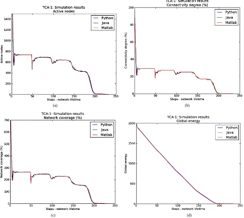
Figure 6 shows a comparison of Matlab, Java and Py- thon implementations based on the simulation results of TCA-1 via a cellular automaton with a Moore neigh- bourhood. It can be seen that the use of a different pro-
gramming environment does not affect performance of the WSN in terms of network lifetime (Figure 6(a)), connectivity (Figure 6(b)), coverage (Figure 6(c)) and global energy (Figure 6(d)).
However, the programming environment does affect 1) the size of the WSN used for simulation purposes 2) the visualization of simulation results and 3) how easy it is for a new researcher to use a programming environment in order to conduct simulations using cellular automata.
Matlab can efficiently support large network sizes (e.g., WSN of at least 250.000 sensors). However, it is rather inefficient for the development of GUI-based simula- tions and rather hard to learn for a researcher with only
(a) (b)
(c) (d)
Figure 6. Simulation results: TCA-1 active nodes, connectivity, coverage and global energy (CA with a Moore neighbour-hood). (a): Simulation results: TCA-1 active nodes (CA with Moore neighbourhood); (b): Simulation results: TCA-1 connec-tivity (CA with Moore neighbourhood); (c): Simulation results: TCA-1 coverage (CA with a Moore neighbourhood); (d):
imulation results: TCA-1 global energy (CA with a Moore neighbourhood). S
basic programming knowledge. Java can efficiently sup- port large enough network sizes (e.g., WSN of approxi- mately 22.500 sensors) and, in addition, it can simplify the design and development of GUI-based simulations, demanding, however, a sophisticated (thus costly) com- puting system. Java is a programming environment quite easy to learn and should be preferred by researchers with basic programming skills. Python can be a good choice for simulating small WSN (e.g., WSN of at most 6.500 sensors) and a perfect choice for the development of user-friendly GUI-based simulations. Note that Python can be used for simulations involving very large WSN as well, but lacks efficiency when it comes to visualization. Python is an easy-to-learn and very flexible program-
ming environment and certainly makes a perfect choice for researchers no matter how skilled they are in terms of programming.
4.1. TCA-1 Simulation Results
[image:8.595.57.538.263.679.2]The following simulations have been implemented using the Python programming environment.
Figure 7 shows simulation results for algorithm TCA-1 via cellular automata with 1) a Margolus neigh- bourhood with at most 1 (l = 1) active sensors in each neighbourhood, 2) a Margolus neighbourhood with at most 2 (l = 2) active sensors in each neighbourhood) and 3) a Weighted Margolus neighbourhood.
(a) (b)
(c) (d)
It is observed that a cellular automaton with a Mar- go
Figure 8 shows simulation results for algorithm TC
Weighted lus neighbourhood with at most 2 (l = 2) active sensors
in each neighbourhood results in poor performance of TCA-1 in terms of network lifetime (Figure 7(a)) and global energy (Figure 7(d)). This is reasonable since the increased redundancy in active nodes causes the global energy of the network to drop very fast; on the other hand, as a natural consequence, a very good connectivity level is obtained (Figure 7(c)). However, using a cellular automaton with a Weighted Margolus neighbourhood leads to a very good performance of TCA-1: prolonga- tion of the network lifetime together with good connec- tivity and coverage levels.
A-1 via cellular automata with 1) a Block neighbour- hood with at most 1 (l = 1) active sensors in each neighbourhood, 2) a Block neighbourhood with at most 2 (l = 2) active sensors in each neighbourhood and 3) a Weighted Block neighbourhood. Simulation results fol- low the same fashion as before (i.e., when cellular auto- mata with variations of a Margolus neighbourhood are used): using a cellular automaton with a Weighted Block neighbourhood leads to a very good performance of TCA-1: prolongation of the network lifetime together with good connectivity and coverage levels.
Based on the observation that the use of
(a) (b)
(c) (d)
Figure 8. Simulation results: TCA-1 active nodes, connectivity, coverage, global energy (CA with variations of a Block neigh- bourhood). (a): Simulation results: TCA-1 active nodes (CA with variations of Block neighbourhood); (b): Simulation results: TCA-1 connectivity (CA with variations of Block neighbourhood); (c): Simulation results: TCA-1 coverage (CA with varia-tions of Block neighbourhood); (d): Simulation results: TCA-1 global energy (CA with variavaria-tions of Block neighbourhood).
argolus or Weighted Block neighbourhoods in the cor- ment make better decisions on whether to remain activ
M e
4.2. TCA-2 Simulation Results
s have been imple-
go- rit
responding cellular automata results in improved per- formance of algorithm TCA-1, we present simulation results for the performance of TCA-1 in terms of active sensors and global energy (Figure 9) as well as connec- tivity and coverage (Figure 10) obtained through simula- tions using cellular automata with the following neighbouring schemes: Moore, von Neumann, Weighted Margolus, Weighted Block and Slider; the case when no topology control algorithm is used is also depicted. It is observed that the use of cellular automata with a Moore, Weighted Margolus or Slider neighbourhood raises the best performance of TCA-1 algorithm. Conclusion/rec- ommendation: in order to obtain efficient simulations of topology control algorithms in WSN, cellular automata neighbourhoods should capture the fact that when nodes have increased knowledge of their surrounding environ-
or idle.
Similarly, the following simulation
mented using the Python programming environment.
Figures 11 and 12 show simulation results for al hm TCA-1 via cellular automata with 1) a Moore neighbourhood and 2) a Weighted Margolus neighbour- hood in comparison with algorithm TCA-2 via a cellular automaton with a Moore neighbourhood in terms of ac- tive nodes, global energy, coverage and connectivity; the case when no topology control algorithm is used is also depicted. It is observed that the (weak) randomization used by TCA-2 leads to (slightly) improved results (compares to the deterministic TCA-1) as far as network lifetime, coverage and connectivity are concerned.
[image:10.595.65.536.302.495.2]
(a) (b)
Figure 9. Simulation res ourhood schemes).
ults: TCA-1 active sensors (a) and global energy (b) (CA with different neighb
(a) (b)
Figure 10. Simulation re od schemes).
[image:10.595.61.538.523.716.2]
[image:11.595.63.535.83.288.2]
(a) (b)
Figure 11. Simulation resu ighbourhood and a
lts: TCA-2 (CA with a Moore neighbourhood) vs TCA-1 (CA with a Moore ne Weighted Margolus neighbourhood) active sensors (a) and global energy (b).
(a) (b)
Figure 12. Simulation resu ighbourhood and a
We have used cellular automata for simulating and
determine how the selection of a neighbourhood in cel-
hms; th
lts: TCA-2 (CA with a Moore neighbourhood) vs TCA-1 (CA with a Moore ne Weighted neighbourhood) coverage (a) and connectivity (b).
5. Conclusions
evaluating two topology control algorithms in WSN us- ing Matlab, Java and Python programming environments. Both algorithms are based on the selection of an appro- priate subset of sensor nodes that must remain active in order to increase network lifetime, maintaining adequate levels of connectivity and coverage; one of them deter- ministically selects the subset of active nodes while the other uses a weak random source in order to select which nodes should remain active. In our simulations, we have experimentally investigated different neighbouring sche- mes for the corresponding cellular automata in order to
lular automata models can affect the performance of simulation of topology control algorithms in WSN.
Even the use of weak randomization seems to improve the performance of simple topology control algorit
[image:11.595.60.537.327.531.2]experimentally evaluate my ideas from scratch: what it would be best to use: Matlab, Java or Python”, the an-swer is not straightforward. Focusing on the necessary network size, Matlab and Java offer the best support. If GUI-based simulations are needed, then Java and Python should be considered. However, for small scale GUI- based simulations involving cellular automata, Python certainly makes a simple, cost-effective and efficient programming environment.
REFERENCES
[1] J. V. Neuman Reproducing
mata,” (Edited . Burks), Univer
e
dge University Press,
Cam-ic Publishing Co. Pte. Ltd, London, 2001.
Singapore City, 1986.
26-829. n, “The Theory of
and Completed by A. W
Auto -sity of Illinois Press, Urbana and London, 1966. [2] M. Gardner, “The Fantastic Combinations of John
Con-way’s New Solitaire Game ‘Life’,” Scientific Am rican, Vol. 223, 1970, pp. 120-123.
[3] B. Chopard and M. Droz, “Cellular Automata Modeling of Physical Systems,” Cambri
bridge, 1998.
[4] A. Ilachinski, “Cellular Automata: A Discrete Universe,” World Scientif
[5] S. Wolfram, “A New Kind of Science,” Wolfram Media, Inc., Champaign, 2002.
[6] S. Wolfram, “Theory and Applications of Cellular Auto-mata,” World Scientific,
[7] M. Nowak and R. May, “Evolutionary Games and Spatial Chaos,” Nature, Vol. 359, No. 6398, 1992, pp. 8
doi:10.1038/359826a0
[8] B. Applebaum, Y. Ishai and E. Kushilevitz, “Crypto- graphy by Cellular Automata or How Fast Can Com
A Cellular Learning
Auto-a,”
escribing a Biological Immune System,” plex- ity Emerge in Nature?” Proceedings of the 1st Symposium on Innovations in Computer Science (ICS 10), Beijing, 5-7 January 2010, pp. 1-19.
[9] H. Beigy and M. R. Meybodi, “A Self-Organizing Chan- nel Assignment Algorithm:
mata Approach,” Intelligent Data Engineering and Auto- mated Learning, Vol. 2690, 2003, pp. 119-126.
[10] N. Ganguly, B. K. Sikdar, A. Deutsch, G. Canright and P. Pal Chaudhuri, “A Survey on Cellular Automat Tech- nical Report, Centre for High Performance Computing, Dresden University of Technology, Dresden, 2003. [11] A. Boondirek, W. Triampo and N. Nuttavut, “A Review
of Cellular Automata Models of Tumor Growth,” Inter- national Mathematical Forum, Vol. 5, No. 61, 2010, pp. 3023-3029.
[12] T. Tome and J. R. D. De Felicio, “Probabilistic Cellular Automata D
Physical Review E, Vol. 53, No. 4, 1996, pp. 3976-3981. doi:10.1103/PhysRevE.53.3976
[13] P. Sloot, F. Chen and C. Boucher, “Cellular Automaton Model of Drug Therapy for HIV Infection,” Proceedings
t through Cellular Automaton
of the 5th International Conference on Cellular Automata for Research and Industry (ACRI 02), Geneva, 9-11 Oc-tober 2002, pp. 282-293.
[14] G. Iovine, S. Di Gregorio and V. Lupiano, “Debris-Flow Susceptibility Assessmen
Modeling: An Example from 15-16 December 1999 Dis- aster at Cervinara and San Martino Valle Caudina (Cam- pania, Southern Italy),” Natural Hazards and Earth Sys- tem Sciences, Vol. 3, 2003, pp. 457-468.
doi:10.5194/nhess-3-457-2003
[15] M. Mitchell, P. T. Hraber and J. P. Crutche the Edge of Chaos: Evolving C
ld, “Revisiting ellular Automata to
Per-ata,” Proceedings of the 7th AGILE
Movement Model
Con-ta for Topology Con-
r Topology Control
g
ed Models of Wireless Sensor Networks,”
sing Cell-DEVS,” Pro-
ology Control
rence through Topology Control,” Algo-form Computations,” Complex Systems, Vol. 7, No. 2, 1993, pp. 89-130.
[16] H. Demirel and M. Cetin, “Modelling Urban Dynamics via Cellular Autom
Conference on Geographic Information Science, Haifa, 15-17 March2010, pp. 313-323.
[17] L. Z. Yang, W. F. Fang, J. Li, R. Huang and W. C. Fan, “Cellular Automaton Pedestrian
sidering Human Behavior,” Chinese Science Bulletin, Vol. 48, No. 16, 2003, pp. 1695-1699.
[18] S. Athanassopoulos, C. Kaklamanis, G. Kalfountzos and E. Papaioannou, “Cellular Automa
trol in Wireless Sensor Networks using Matlab,” Pro- ceedings of the 7th FTRA International Conference on Future Information Technology (FutureTech 12), Van-couver, 26-28 June2012, pp. 13-21.
[19] S. Athanassopoulos, C. Kaklamanis, P. Katsikouli and E. Papaioannou, “Cellular Automata fo
in Wireless Sensor Networks,” Proceedings of the 16th Mediterranean Electrotechnical Conference (Melecon 12), Yasmine Hammamet, 25-28 March 2012, pp. 212-215. [20] R. O. Cunha, A. P. Silva, A. A. F. Loureiro and L. B.
Ruiz, “Simulating Large Wireless Sensor Networks usin Cellular Automata,” Proceedings of the 38th Annual Simulation Symposium, Washington DC, 4-6 April 2005, pp. 323-330.
[21] W. Li, A. Y. Zomaya, and A. Al-Jumaily, “Cellular Automata Bas
Proceedings of the 7th ACM International Symposium on Mobility Management and Wireless Access (MobiWAC 09), New York, 2009, pp. 1-6.
[22] B. Qela, G. Wainer and H. Mouftah, “Simulation of Large Wireless Sensor Networks u
ceedings of the 2009 Winter Simulation Conference, Aus- tin, 13-16 December 2009, pp. 3189-3200.
[23] W. Zhang, L. Zhang, J. Yuan, X. Yu and X. Shan, “Demonstration of Non-Cluster Based Top
Method for Wireless Sensor Networks,” Proceedings of the 6th IEEE Consumer Communications and Networking Conference (CCNC 2009), Las Vegas, 10-13 January 2009, pp. 1-2.
[24] T. Lou, H. Tan, Y. Wang and F. C. M. Lau, “Minimizing Average Interfe
rithms for Sensor Systems, Vol. 7111, 2012, pp. 115-129. [25] P. Santi, “Topology Control in Wireless Ad-Hoc and
Sensor Networks,” ACM Computing Surveys, Vol. 37, No. 2, 2005, pp. 164-194. doi:10.1145/1089733.1089736 [26] M. Burkhart, M., P. von Rickenbach, R. Wattenhofer and
ence?” Proceedings of the 5th ACM International Sympo- sium on Mobile ad hoc Networking and Computing (Mo- biHoc 2004), New York, ACM, 2004, pp. 9-19.
doi:10.1145/989459.989462
[27] T. Johansson and L. Carr-Motyckova, “Reducin ference in Ad Hoc Networks
g Inter-through Topology Control,”
With Companion
Simula-Cellular Automata: A Discrete View of the World
g, “Greedy Perimeter Stateless
er,
a,
ong, S. Lu and L. Zhang, “Energy Efficient Rout
Proceedings of the 2005 Joint Workshop on Foundations of Mobile Computing (DIALM-POMC 2005), New York, 2005, pp. 17-23.
[28] M. A. Labrador and P. M. Wightman, “Topology Control in Wireless Sensor Networks:
“Geo
tion Tool for Teaching and Research,” Springer, Berlin, 2009.
[29] J. L. Schiff, “Partitioning Cellular Automata,” In: J. L.
Schiff, ,
“G
John Wiley and Sons, Inc., Hoboken, 2008, pp. 115-116. [30] T. Toffoli and N. Margolus, “The Margolus
Neighbour-hood,” In: Cellular Automata Machines: A New
Envi-ronment for Modeling,MIT Press in Scientific Computa-tion, 1987, pp. 119-138.
[31] B. Karp and H. T. Kun
ing for Wireless Networks,” Proceedings of the 6th Annual International Conference on Mobile Computing and Networking, New York, 2005, pp. 243-254.
[32] F. Kuhn, R. Wattenhofer, Y. Zhang and A. Zolling metric Ad-Hoc Routing: Of Theory and Practice,” Proceedings of the 22nd Annual Symposium on Principles of Distributed Computing, New York, 2003, pp. 63-72. [33] A. Rao, Ch. Papadimitriou, S. Shenker and I. Stoic
eographical Routing without Location Information,” Proceedings of the 9th Annual International Conference on Mobile Computing and Networking, New York, 2003, pp. 96-108.
[34] F. Ye, G. Zh