A Generalized Elastic Net Regularization with Smoothed l0 Penalty

http://www.scirp.org/journal/apm ISSN Online: 2160-0384

ISSN Print: 2160-0368

A Generalized Elastic Net Regularization with

Smoothed

_

₀

Penalty

Sisu Li, Wanzhou Ye

Department of Mathematics, College of Science, Shanghai University, Shanghai, China

Abstract

This paper presents an accurate and efficient algorithm for solving the generalized elastic net regularization problem with smoothed 0 penalty for

recovering sparse vector. Finding the optimal solution to the unconstrained

0

 minimization problem in the recovery of compressive sensed signals is an NP-hard problem. We proposed an iterative algorithm to solve this problem. We then prove that the algorithm is convergent based on algebraic methods. The numerical result shows the efficiency and the accuracy of the algorithm.

Keywords

Sparse Vector, Compressed Sense, Elastic Net Regularization,

0

 Minimization

1. Introduction

Compressive sensing (CS) has been emerging as a very active research field and brought about great changes in the field of signal processing during recent years with broad applications such as compressed imaging, analog-to-information conversion, biosensors, and so on [1] [2][3]. Meanwhile, the 0 norm based

signal recovery is attractive in compressed sensing as it can facilitate exact recovery of sparse signal with very high probability [4][5]. Mathematically, the problem can be presented as

0

min , subject to ,

N

x R

x Ax y

∈ = (1)

where y∈Rm,A∈Rm N× is a measurement matrix, 2

⋅ _{denotes the Euclidean}

norm and x0, formally called the quasi-norm, denotes the number of the

nonzero components of

(

)

T

1, 2, ,

N n

x= x x  x ∈R , and the λ>0 is a regulari-

zation parameter. How to cite this paper: Li, S.S. and Ye,

W.Z. (2017) A Generalized Elastic Net Regularization with Smoothed 0

Penal-ty. Advances in Pure Mathematics, 7, 66- 74.

http://dx.doi.org/10.4236/apm.2017.71006

Received: December 6, 2016 Accepted: January 21, 2017 Published: January 24, 2017

Copyright © 2017 by authors and Scientific Research Publishing Inc. This work is licensed under the Creative Commons Attribution International License (CC BY 4.0).

We can then solve the unconstrained 0 regularization problem

2

2 0

1

min ,

2

N x R

Ax y λ x

∈

 _{− +} 

 

  (2)

A natural approach to this problem is to solve a convex relaxation 1 re-

gularization problem [6][7] as following

2

2 1

1

min ,

2

N x R

Ax y λ x

∈

 _{− +} 

 

  (3)

where the 1 1

N i i

x =

∑

₌ x is the 1 norm. Undoubtly, the 1 regularization

has many applications [8][9] and can be solved by many classic algorithms such as the iterative soft thresholding algorithm [7], the LARs [10], etc. An effective regression method, Lasso [11], has a very close relationship with the 1 re-

gularization as well. In 2005, Zou et al. proposed the following algorithm, which called the elastic net regularization [12]

2

1 2

2 1 2

1

min ,

2

N x R

Ax y λ x λ x

∈

 _{− + +} 

 

  (4)

where the λ λ >1, 2 0 are two regularization parameters. It is proved in many

papers that the elastic net regularization outperforms the Lasso in prediction accuracy. Cands proved that as long as A satisfies the RIP condition with a constant parameter, the 1 minimization can yield an equivalent solution as

that of 0 minimization [13]. So in general, the 1 regularization problem can

be regard as an aproach to the 0 regularization. Therefore, we shall consider a

generalized elastic net regularization problem with 0 penalty:

2 2

1 2

2 0 2

1

min ,

2

N x R

Ax y λ x λ x

∈

 _{− + +} 

 

  (5)

Unfortunately, the 0 norm minimization problem is NP-hard [14]. And

due to the sparsity of the solution x, we could turn out to calculate the following generalized elastic net regularization with smoothed 0 penalty:

2 2

1 2

2 0, 2

1

min ,

2

N x R

Ax y λ x _δ λ x

∈

 _{− + +} 

 

  (6)

where 0, 1 2 2

N _i

i i

x x

x

δ =

∑

= _+δ , the δ >0 is a parameter which approaches zero in

order to approximate x0.

In this paper,we propose an iterative algorithm for recovering sparse vectors which substitute the 0 penalty with a function [15]. And by adding an 2

term, we can prove that the algorithm is convergent based on the algebraic methods. In the experiment part, we compare the algorithm with the 1 soft

thresholding algorithm (ITH) [16]. And the output results show an outstanding success of the new method.

Section 5.

2. Problem Reformulation

The reconstruction method discussed in this paper is for directly approaching the l0 norm and obtaining its minimal solution with suitably designed

objective functions. We denote by Cδ

(

x,λ λ1, 2

)

the objective function of the

minimization problem (6).

(

)

2 2 2

1 2 2 1 2 2 2

1

1

, , .

2

N i

i i x

C x Ax y x

x

δ λ λ λ _δ λ

=

= − + +

+

∑

(7)

Our goal is to minimize the objective function. For any δ >0 and λ λ >1, 2 0,

the minimization problem is convex coercie, thus it has a solution. So the optimal solution of (7) can be given according to the optimal condition.

(

)

(

)

T 1

2 2

2 1

ˆ 2

ˆ 2 ˆ 0.

ˆ

i

i

i N

x

A Ax y x

x

λ δ _λ

δ ≤ ≤

 

 

− + + =

 ₊ 

 

 

(8)

Then we can present the following iterative algorithm to solve the above minimization problem.

Algorithm 1 Iterative Algorithm for Generalized Elastic Net Regularization with Smoothed 0

Penalty (IAGENR-L0)

0: Given vector y, matrix A, choose parameters δ>0,λ λ1, 2>0 and initialize 0 N

x ∈R

1: for k=1 do

2: Compute the following system for ( )k1

x +

( )

(

)

(

)

1

1 T 1 1

2 2

2

1

2

2 0

k

j k k

k j

j N

x

A Ax y x x

λ δ

λ δ

+

+ +

≤ ≤

 

  _{+ − + =}

 

+

 

 

(9)

3: Or compute the equivalent equation

( )

(

)

T 1 1 T

2 2

2

Diag , 1, 2, , k

k i

A A i N x A y

x

λ δ δ

+

  

 ₊  ₌  ₌

  

+

 _ _

 

 (10)

4: Stop when 1 2

k k

x+ −x <δ

5: end for

6: Output the vector 0 N

x ∈R

3. Convergence of the Algorithm

In this section, we prove that the algorithm is convergent. Firstly, we start from the lemma 1 [17] which we can deduce the inquality directly by using the mean value theorem.

Lemma 1. Given δ >0 , then the inequality

(

)

(

)

(

(

)

)

2

2 2

2 2 2 2

2 2

2 x y y x y

x y

x y _{x x}

δ δ

δ δ _{δ δ}

− −

− − ≥

+ + _{+ +} (11)

Proof. We first denote

( )

2 2 2 x f x x δ =

+ , then by the mean value theorem, we

have

( ) ( )

2 2

( )

(

2 2

)

_{where between} 2 _and 2_.

f x − f y = f′ ξ x −y ξ x y (12)

So we have

(

)

(

)

(

)

(

)

(

)

2 2 2

2 2

2 2 2 2

2

2

.

x y x y y x y

x y

x y _x

δ _{δ δ}

δ δ ξ δ _δ

− − + −

− = =

+ + + + (13)

Thus, we can simplify the inequality as follow:

(

)

(

)

(

(

)

)

2 2 2

2 2

2 2 2 2

2 2

2

.

x y x y

x y

x y _{x x}

δ _δ

δ δ _{δ δ}

− ₋

− − ≥

+ + _{+ +}

This inequality of (11) holds no matter 2 2

x >y , x2 < y2 or x2 = y2. And

the next Lemma proves that the sequence ( )k

x drives the function Cδ

(

x,λ λ1, 2

)

downhill. □ Lemma 2. For any δ >0 and λ λ >₁, ₂ 0, let x(k+1) be the solution of (9) for

1, 2, 3,

k=  Then we can have

(

)

(

)

(

)

2

1 1

1 2 1 2

2 2 , , , , .

k k k k

Ax −Ax + ≤ C_δ x λ λ −C_δ x + λ λ (14)

Furthermore,

(

)

(

)

(

)

2

1 1

1 2 1 2

2 , , , , .

k k k k

x −x + ≤c C_δ x λ λ −C_δ x+ λ λ (15)

where c is a positive constant that depends on λ2.

Proof.

(

)

(

)

( )

( )

( )

( )

(

)

( )

( )

( )

( )

(

)

(

)

2 2 1 1

1 2 1 2 1 2 ₁ 2

1

2 ₁2 2 ₁ 2

2 _{2 2 2 2}

2 ₁ 2

1 2 ₁ 2

1 2 2 1 1 2 2 2 T

1 1 1

2 , , , , 1 ( ) 2 1 2 2 k k N i i k k k k i i i

k k k k

k k N i i k k i i i

k k k k

k k k k k

x x

C x C x

x x

x x Ax y Ax y

x x

x x

Ax Ax x x

x x x Ax Ax

δ λ λ δ λ λ λ

δ δ λ λ δ δ λ λ + + + = + + + + = + + + + +     − = _ − _  + +    + − + − − −     = _ − _  + +    + − + − + − + −

∑

∑

(

)

T 1 . k Ax+ −y

(16)

Using (9). The last term in (16) can be simplified to be

(

) (

) (

) ( )

( )

(

)

(

)

( )

(

)

(

)

1

T T 1

1 1 1 1 1

2 ₂ 2

1 1

1 _{1 1}

2 2 2 1 2 2 2 2 . k

k k k k k T k

k

k k k

N _T

i i i _{k k k}

i k

x

Ax Ax Ax y Ax Ax A x

x

x x x

x x x

Substituting (15) into (16) and using (11),

(

)

(

)

( )

( )

( )

( )

(

_{( )}

(

)

)

(

)

( )

(

)

1

1 2 1 2

2 ₁ 2 _{1 1}

1 2 ₁ 2 ₂ 2

1 2 2 1 1 2 2 2 2 1 2 2

1 _{1 1}

2

2 _{2 2}

2 1 , , , , 2 1 2 1 . 2 k k

k k k k k

N

i i i i i

k k

i k

i i

k k k k

k k

N

i _{k k k k}

i k

C x C x

x x x x x

x x _x

Ax Ax x x

x x

Ax Ax x x

x

δ λ λ δ λ λ

δ λ

δ δ _δ

λ δλ λ δ + + + + + = + + + + + = −    −  =  − −   + + ₊      + − + − − ≥ + − + − +

∑

∑

(18) □

Since

(

)

( )

(

)

2 1 1 2

1 ₂ 0

k k i N i k x x x δλ δ + = − ≥ +

∑

for any k

x and k 1

x + . From (18) we can

obtain the results of (14) and (15) with

2

1

C

λ = _.

Lemma 3. ([18], Theorem 3.1) Let P z w

(

,

)

=0 to be given, and let

( ) ( )

(

, ,

)

0

Q z a c = be its corresponding highest ordered system of equations. If

( ) ( )

(

, ,

)

0

Q z a c = has only the trivial solution z=0, then P z w

(

,

)

=0 has

1

m i i q

β =

∏

₌ solutions, where qi is the degree of Pi.

Theorem 1. For any δ >0 and λ λ >1, 2 0. Then the iterative solutions

k x

in (9) converge to *

x , that is *

lim_k→∞xk =x and x* is a critical point of (6).

Proof. Here, we need to prove that the sequence k

x is bounded. We assume

that _xki is one convergent subsequence of _xk and its limit point is _x*. By (15) we know that the sequence _xki+1 also converges to _x*. If we replace _xk,

1

k

x + with _xki,_xki+1 in (10) and letting _i→ ∞ yields.

□

( )

(

)

(

)

*

1 T * *

2 2 2 * 2 2 0. j j x

A Ax y x

x

λ δ

λ δ

+ − + =

+ (19)

And this implies that the limit point which converges to any convergent subsequence of k

x is the critical point of (8). In order to prove the convergence

of sequence k

x , we need to prove that the limit point set M, which contains all

the limit points of convergent subsequence of k

x is a finite set. So we have to

prove that the following equation has finite solutions.

( )

(

1

)

2 T

(

)

2

2 1 2 2 0. j i i N u

A Au y u

u λ δ λ δ ≤ ≤     _{+ − + =}   +     (20)

where

(

)

T

1, 2, ,

N N

u= u u u ∈R . We can rewrite (20) as follow:

( )

(

1₂

)

2

(

T 2

)

T

1 2 2 0. j N i i N u

A A I u A y

It is obvious that T 2

2 N

A A+ λ I is a positive definite matrix, A yT ∈RN is the N×N identity matrix. Then the (21) can be rewritten as the following eq-

uation:

(

)

(

T T

)

1 2

2λ δu+B A A+2λ IN u−A y =0. (22)

where B is an N×N diagonal matrix with diagonal entries

( )

(

₂

)

2

, 1, 2, 3, ,

ii i

B = u +δ i=  N. We denote A AT +2λ2IN =

( )

aii N N× and

(

)

T

T

1, 2, , N

A y= q q  q . Then

(

)

(

)

(

)

(

)

(

)

(

)

2 2

1 1 11 1 12 2 1 1 1

2 2

1 2 21 1 22 2 2 2 2

2 2

1 1 1 2 2

2 0,

2 0,

2 0.

N N

N N

N N N NN N N N

u a u a u a u q u

u a u a u a u q u

u a u a u a u q u

λ δ δ

λ δ δ

λ δ δ

 _{+ + + + − + =}

 

+ + + + − + =

   

 + + + + − + =





 



(23)

If we want to prove that (23) has finite solutions, then we can prove the (22) system has finite solutions. According to lemma 3, if we prove that the highest ordered system of (23) has only trivial solution, then it's easy to conclude that the Equation (23) has finite solutions.

(

)

(

)

(

)

4 11 1 12 2 1 1 4 21 1 22 2 2 2

4 1 1 2 2

0, 0,

0. N N

N N

N N NN N N

a u a u a u u

a u a u a u u

a u a u a u u

 + + + =

 _{+ + + =}

  

 _{+ + + =}



  



(24)

We prove the system (24) has only trivial solution. We assume that

(

)

T

1, 2, , , 0, , 0

N s

u= u u  u  ∈R is a nonzero solution of (24), ui ≠0 for 1, 2, ,

i=  s, 1≤ ≤s N. Then we have 0. s

Cu = (25)

where C=

( )

aii s s× is the s×s leading principle submatrix of matrix T

2

2 _N

A A+ λ I is the positive definite, therefore the matrix C is positive definite

as well. So we have ui =0 for i=1, 2,,s. This contradicts the assumption of 0

i

u ≠ , i=1, 2,,s, 1≤ ≤i s.

Therefore, the system (24) has only trivial solution. So the Equation (20) has finite solutions. Since all the limit points of convergent subsequence of ( )k

x

satisfies the Equation (20) and we have proved that (20) has finite solutions. So the limit point set M is a finite set. Combining with ( 1) ( )

2

0

k k

x + −x → as

k→ ∞, we thus obtain that the sequence x( )k is convergent and limit *

x is a

critical point of problem (7).

4. Numerical Experiments

In this section, we present some numerical experiments to show the efficiency and the accuracy of the Algorithm 1 for sparse vector recovery. We compare the performance of Algorithm 1 with 1 IST [3]. In the test, the matrix A had the

size of 100 250× , which is m=100 and N=250. All the experiments were

independent trials for various sparsity s.

The experiment results contain two parts: the first one focuses on the comparison of the two algorithms in accuracy; the other one focuses on the efficiency of the two algorithms. In the experiments, the mean squared error of the original vector and the result is recorded as

2 0

2

MSE= _xk−_{x N} (26)

4.1. Comparison on the Accuracy

The matrix 100 250

A∈R × and the original sparse vector x0∈R250 was gene-

rated randomly according to the standard Gaussian distribution with N-length and s-sparse, which varies as 2, 4, 6, 8, ···, 48. The location of the nonzero elements were randomly generated. The regularization parameters were set as

6

10

δ ₌ − _and 3 5

1 10 , 2 10

λ ₌ − λ ₌ − _{. All the other parameters of the two al-}

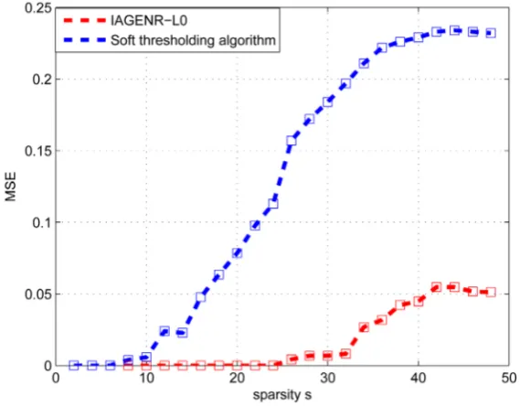
gorithms were set to be the same.The results are shown in Figure 1.

The Figure 1 shows that the convergence error MSE for the two algorithms tends to be stable at last for different sparsity s. We can also observe that the MSE of the LAGENR-L0 is lower than the IST which demonstrates that our algorithm is not only convergent,but also outperforms the IST in accuracy.

4.2. Comparison on the Efficiency

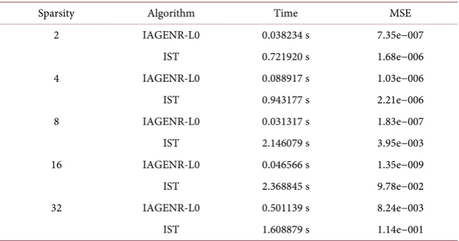
In this subsection, we focus on the speed of the two algorithms. We conduct various experiments to test the effectiveness of the proposed algorithm. Table 1

[image:7.595.232.517.474.696.2]

report the numerical results of the two algorithms for recovering vectors for different sparsity level. From the results, we can see that the IAGENR-L0 performs much better than IST in efficiency and the accuracy.

Figure 1. Comparison of the convergence error 0 2 2

MSE k

x x N

[image:8.595.208.539.88.262.2]

Table 1. The iteration time of the IAGENR-L0 and the IST for different sparsity level.

Sparsity Algorithm Time MSE

2 IAGENR-L0 0.038234 s 7.35e−007

IST 0.721920 s 1.68e−006

4 IAGENR-L0 0.088917 s 1.03e−006

IST 0.943177 s 2.21e−006

8 IAGENR-L0 0.031317 s 1.83e−007

IST 2.146079 s 3.95e−003

16 IAGENR-L0 0.046566 s 1.35e−009

IST 2.368845 s 9.78e−002

32 IAGENR-L0 0.501139 s 8.24e−003

IST 1.608879 s 1.14e−001

5. Conclusion

In this paper, we consider an iterative algorithm for solving the generalized elastic net regularization problems with smoothod 0 penalty for recovering

sparse vectors. Then a detailed proof of convergence of the iterative algorithm is given in Section 2 by using the algebraic method. Additionally, the numerical experiments in Section 3 show that our iterative algorithm is convergent and performs better than the IST on recovering sparse vectors.

References

[1] Donoho, D.L. (2006) Compressed Sensing. IEEE Transactions on Information Theory, 52, 1289-1306.

[2] Cands, E.J., Romberg, J. and Tao, T. (2006) Robust Uncertainty Principles: Exagct signal Reconstruction from Highly Incomplete Frequency Information. IEEE Transactions on Information Theory, 26, 489-509.

[3] Duarte, M.F. and Eldar, Y.C. (2011) Structured Compressed Sensing: From Theory to Applications. IEEE Transactions on Signal Processing, 59, 4053-4085.

[4] Lu, Z. (2014) Iterative Hard Thresholding Methods for 0 Regularized Convex

cone Programming. Mathematical Programming, 147, 125-154. https://doi.org/10.1007/s10107-013-0714-4

[5] Cand‘es, E.J. and Tao, T. (2005) Decoding by Linear Programming. IEEE Transac-tions on Information Theory, 51, 4203-4215.

[6] Chen, S.S., Donodo, D.L. and Saunders, M.A. (1998) Atomic Decomposition by ba-sis Pursuit. SIAM Journal on Scientific Computing, 20, 33-61.

https://doi.org/10.1137/S1064827596304010

[7] Daubechies, I., Defries, M. and DeMol, C. (2004) An Iterative Thresholding Algo-rithm for Linear Inverse Problems with a Sparsity Constraint. Communications on Pure and Applied Mathematics, 57, 1413-1457.

[8] Zou, H. (2006) The Adaptive Lasso and Its Oracle Properties. Journal of the Ameri-can Statistical Association, 101, 1418-1429.

https://doi.org/10.1198/016214506000000735

https://doi.org/10.1214/07-AOS582

[10] Efron, B., Hastie, T., Johnstone, I. and Tibshirani, R. (2004) Least Angle Regression.

The Annals of Statistics, 32, 407-451.

[11] Tibshirani, R. (1996) Regression Shrinkage and Selection via the Lasso. Journal of the Royal Statistical Society Series B (Statistical Methodology), 73, 273-282.

[12] Zou, H. and Hastie, T. (2005) Regularization and Variable Selection via the Elastic Net. Journal of the Royal Statistical Society Series B (Statistical Methodology), 67, 301-320.

[13] Kordas, G. (2015) A Neurodynamic Optimization Method for Recovery of Com-pressive Sensed Signals with Globally Converged Solution Approximating to L0

Mi-nimization. IEEE Transactions on Neural Networks and Learning Systems, 26, 1363-1374.

[14] Natraajan, B.K. (1995) Sparse Approximation to Linear Systems. SIAM Journal on Computing, 24, 227-234. https://doi.org/10.1137/S0097539792240406

[15] Xiao, Y.H. and Song, H.N. (2012) An Inexact Alternating Directions Algorithm for Constrained Total Variation Regularized Compressive Sensing Problems. Journal of Mathematical Imaging and Vision, 44, 114-127.

[16] Daubechies, I., Defrise, M. and Mol, C.D. (2004) An Iterative Thresholding Algo-rithm for Linear Inverse Problems with a Sparsity Constraint.

[17] Lai, M.J., Xu, Y.Y. and Yin, W.T. (2013) Improved Iteratively Reweighted Least Squares for Unconstrained Smoothed Lq Minimization. SIAM Journal on

Numeri-cal Analysis, 51, 927-957.

[18] Garcia, C.B. and Li, T.Y. (1980) On the Number of Solutions to Polynomial Systems of Equations. SIAM Journal on Numerical Analysis, 17, 540-546.

https://doi.org/10.1137/0717046

Submit or recommend next manuscript to SCIRP and we will provide best service for you:

Accepting pre-submission inquiries through Email, Facebook, LinkedIn, Twitter, etc. A wide selection of journals (inclusive of 9 subjects, more than 200 journals)

Providing 24-hour high-quality service User-friendly online submission system Fair and swift peer-review system

Efficient typesetting and proofreading procedure

Display of the result of downloads and visits, as well as the number of cited articles Maximum dissemination of your research work

Submit your manuscript at: http://papersubmission.scirp.org/