Journal of the Statistical and Social Inquiry Society of Ireland Vol. XXXVIII
TOWARDS REGIONAL ENVIRONMENTAL ACCOUNTS FOR IRELAND
Richard S.J. Tola,b,c , Nicola Comminsa, Niamh Crillya, Seán Lyonsa and Edgar Morgenrotha1
a Economic and Social Research Institute, Whitaker Square, Sir John Rogerson‟s Quay, Dublin 2, Ireland
b
Institute for Environmental Studies, Vrije Universiteit, Amsterdam, The Netherlands
c Department of Spatial Economics, Vrije Universiteit, Amsterdam, The Netherlands
(read before the Society, March 10th, 2009)
__________________________________________________________
Abstract: Existing environmental accounts for the Republic of Ireland are at the national level. This is fine for
continental and global environmental problems, but information at a finer spatial scale is needed for local environmental problems. Furthermore, the impact of environmental policy may differ across space. We therefore construct regional estimates of the environmental pressures posed by Irish households and the environmental problems faced by them. The basic unit of analysis is the electoral district, and the prime data source is the CSO‘s Small Area Statistics, a product of the Census. We use the results of classifying regressions of the Household Budget Survey to impute domestic energy use. We use engineering relations to impute transport fuel use, and secondary data on household behaviour to impute waste arisings. We use EPA data on drinking water use and quality by county. The results show marked regional differences. Electricity use and waste arisings are higher in the East and in the cities and towns. Transport fuel use is highest in the commuter belts around the cities and towns. Other energy is relatively uniform. There is no clear pattern in estimated drinking water use, which may be due to data quality. Drinking water quality is poor across much of the country, but different counties suffer from different problems. The regional estimates are constructed using data in the public domain. However, various government agencies hold data that would allow for the construction of more detailed, more accurate, and more extensive regional environmental accounts.
Keywords: Regional accounts; environmental accounts; energy use; transport; household waste; drinking water quality; drinking water quantity
JEL Classifications: Q52, Q53, Q56
1. INTRODUCTION
Environmental accounts for the Republic of Ireland have been presented at the national scale. This makes sense for some emissions – e.g., it does not matter whether greenhouse gases are emitted in Wexford or in Donegal – but other environmental problems have a clear regional dimension – e.g., drinking water is typically sourced locally, and a clean Liffey does not help the people of Galway. Furthermore, environmental policy may have a different impact on different regions. Therefore, this paper presents estimates of energy use, waste, and water use for over 3,400 electoral districts in the Republic of Ireland.
Regional data on waste generation and water use are obviously important. These services are provided by local authorities. Average levels of provision contain little information. Overcapacity in Cork does not cancel
1
out undercapacity in Limerick. Spatial data on energy use are important for planning the grid, and provide information on the distribution of the impact of policy measures to reduce greenhouse gas emissions. Data on local emissions and resource use may also be used to assess the sustainability of specific settlements or settlement patterns (see for example Moles et al., 2008).
Most of the regional estimates presented in this paper are not directly observed. Rather, the ―data‖ presented here are imputed from things that are observed (by the Census) at regional level and relationships derived from secondary data. Such imputation cannot be avoided. The alternative is to have no regional estimates at all.
Our imputation method uses household microdata to estimate statistical relationships between household characteristics and the variables of interest (i.e. emissions and resource use), and then apply these relationships to the average socioeconomic characteristics of small geographical areas to predict the values that the variables of interest should take in each area. We keep the regressions as simple as possible, often only averaging across multiple household characteristics. We avoid double imputation, that is, we only feed observations into the regression models. We do not use imputed data in the imputation.
Development of regional environmental accounting is in its infancy, but there are several international examples of its application: see e.g. New Zealand Centre for Ecological Economics, 1999 (Northern New Zealand); Turner, 2006 (Jersey); OECD, 2007 (Hyogo Prefecture, Japan); Wadeskog and Eriksson, 2004 (Stockholm); and RAMEA, 2008 (Italy, Netherlands, Poland and the UK).
The paper proceeds as follows. Section 2 discusses the population and income patterns that drive most of our results. Section 3 presents the methods and results for energy use, Section 4 for waste, and Section 5 for water use. Section 6 presents some further analysis that helps to support the conclusions and policy implications. The data can be accessed at:
http://www.esri.ie/irish_economy/environmental_accounts/index.xml
2. POPULATION AND INCOME
Our small area income estimates are derived using two different CSO data sets. The Census yields the Small Area Population Statistics (SAPS), which contain demographic data on household structure, age, education, and employment by electoral district (ED) as well as data on housing conditions and facilities. The Household Budget Survey (HBS) has similar data on housing and demographics plus data on income and expenditures. To impute incomes for each area, we ran a regression of household income in the 2004/5 HBS anonymised data file on the characteristics found in the 2006 SAPS, and used the estimated equation to impute the income level for each electoral district. Because the SAPS hold fairly basic information only, the regression essentially computes the average income in each group. It is a ―classifying regression‖ rather than a continuous function – that is, the explanatory variables are dummies. Table A1 shows the estimated coefficients.
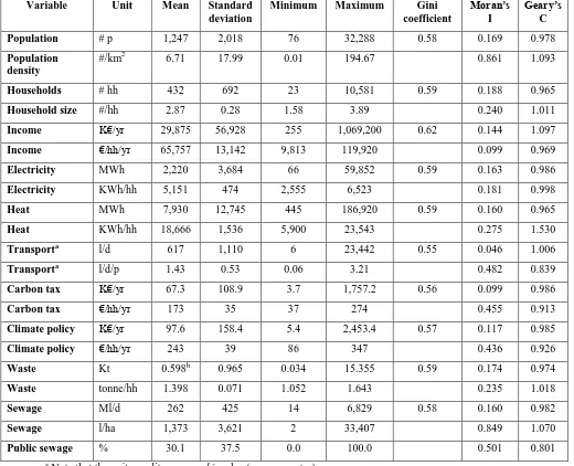
Table 1 shows selected characteristics of the population data by ED. EDs vary widely in the number of people and household that live there, as well as in population density. As revealed by the Gini coefficient, a small number of EDs account for most of the population. Moran‘s I shows that large and densely populated EDs tend to cluster together. The variation in household size is much less, but here we also see spatial agglomeration of small and large households. Figure 1 shows this. Rural households in the west and northwest of the country tend to be smaller than the average. Nonetheless, Table 3 shows a negative correlation between household size and population density.
3. ENERGY, TRANSPORT AND CARBON DIOXIDE EMISSIONS
Regional data on electricity use and other fuel consumption are derived from the SAPS and the HBS, using the same type of classifying regression as described above for household income. Tables A2 and A3 shows the estimated coefficients for electricity use and other fuel consumption, respectively. Other fuels are primarily used for home heating, although there is also some fuel used for lawnmowers and barbeques. However, electricity is also used for heating: in 2005 about 7% of households used electricity as their principal means of winter space heating (Central Statistics Office, 2006, Table 9).
3.1. Energy use
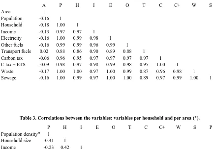
Figure 3 depicts electricity use per household. The spatial pattern lies somewhere in between that of household size (Figure 1) and household income (Figure 2), but differences are less pronounced. This is also seen in Table 1. Table 3 shows that household size is slightly more important than income in explaining electricity use.
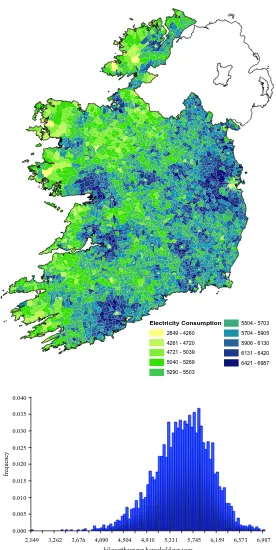
Figure 4 shows fuel consumption for home heating and other purposes per household.2 This is roughly equal across the country – with the exception of a few urban electoral districts, where a combination of small dwellings and fuel poverty leads to heat use that is well below the national average. The positive value of Moran‘s I in Table 1 is explained by the urban concentration of low per household heat use. Table 1 also shows the characteristics of total heat. The concentration of heat use in a few EDs follows the distribution of the population. Income is less important (cf. Table 3).
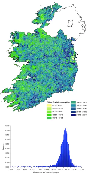
Figure 5 shows transport fuel consumption, for commuting, per adult. The map reveals the commuter belts around the cities – but also shows that these belts are not continuous. Moran‘s I in Table 1 confirms the strong spatial concentration of transport fuel use. The Gini coefficient in Table 1 again reveals that a minority of electoral districts dominate total fuel use – following the distribution of population and work. Table 3 shows that the correlations of transport fuels use to household size and income are indeed low (but positive), while the correlation with population density is negative (and larger, in absolute terms, than any other correlation.) Unfortunately, there is no data available on total transport fuel use.
3.2. The impact of regulation
Figure 3 shows the spatial distribution of electricity use. To a first approximation, Figure 3 also shows the spatial distribution of changes in the price of electricity. These include the price effects of the priority dispatch of peat power and the feed-in tariffs for wind power. In the future, the price of electricity may reflect the price of carbon permits. Similarly, Figure 4 also shows the spatial pattern of the impact of excise duties on heating fuel, and Figure 5 shows the pattern for excises on transport fuel.
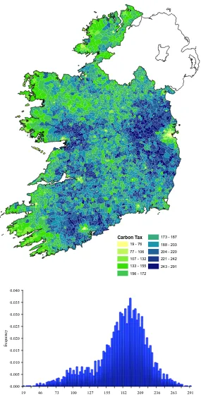
A carbon tax may well be introduced in the foreseeable future, applied to all carbon dioxide emissions that are not already regulated by the EU Emissions Trading Scheme (ETS). Figure 6 shows the average impact per household for each of the electoral districts. Figure 6 is the weighted sum of Figures 4 and 5, with the emission coefficients of heating and transport fuels as weights.3 In the short run, the spatial pattern in Figure 6 is independent of the level of the tax.4 We assumed a carbon tax of €20/tCO2.
Although a carbon tax is occasionally portrayed as being an unfair burden on households at the countryside, Figure 6 shows a more nuanced pattern. A carbon tax would particularly hit the commuter belts around Cork,
2 Strictly, non-electric energy use for anything but transport. 3
Note that these emission coefficient are themselves weighted averages of the fuel-specific emission coefficients. This is particularly relevant for home heating, for which a range of different fuels (from peat to gas) are used.
4 In the long run, the pattern would become less pronounced, as behaviour and technology would change
Dublin, Galway and Limerick, while the rest of the rural areas in fact see a below average impact. Table 3 confirms that transport fuel is more strongly correlated with the carbon tax than is other fuel use.
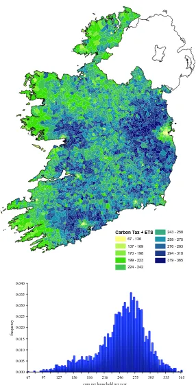
Figure 6 shows the incremental effect of a change in climate policy, viz. the introduction of a carbon tax on non-ETS CO2 emissions. Figure 7 shows the impact of the total package of climate policies, including the
effect of the ETS on electricity prices. That is, Figure 7 adds the carbon dioxide emissions from power generation, assuming that a permit price of €20/tCO2 is fully passed on to final consumers.
Figure 7 reveals a spatial pattern which is less pronounced than that in Figure 6. While Figure 6 suggests that a carbon tax would be spatially inequitable, Figure 7 shows that a carbon tax in fact partially corrects for spatial inequities introduced by the EU ETS.
4. BIODEGRADABLE MUNICIPAL WASTE GENERATED BY HOUSEHOLDS
In this section we estimate the regional distribution of biodegradable municipal waste (BMW) generated by households and subsequently sent to landfill. This waste category is of policy interest because it poses particular problems for the environment if not managed properly and as a consequence is subject to EU regulatory limits.
Purcell and Magette (2009) estimate BMW quantities generated by the household and services sectors in the Dublin area. To estimate household waste, they apply fixed per-household waste generation factors taken from previous studies to SAPS data. Two factors are tested: one based on social class of the household and one based on household size. While both methods provide estimates that are considerably higher than reported aggregate waste generation, the authors find that factors based on household size overstate total waste generation by a smaller margin.
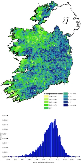
Our approach has some similarities to Purcell and Magette‘s, but rather than building up estimates from per-household factors, we use the relationship between per-household size and waste generation to assign shares of total waste to individual EDs. Following Scott and Watson‘s (2006) results for mixed household waste, we assume that the weight of BMW generated by a household is proportional to the number of people in the household raised to the power 0.486. The number of households by size for each ED is found in the SAPS (see Figure 1). According to the ESRI‘s environmental accounts (based on EPA National Waste Report data), total household BMW sent to landfill in 2006 was 0.95 million tonnes (Lyons et al., 2008).
Figure 8 shows estimated waste per household. Not surprisingly, the pattern is rather similar to the pattern of Figure 1, albeit less pronounced as differences are suppressed by a power that is less than one. Table 3 confirms this. The correlation between household waste and household size is very close to unity.
5. WATER
5.1. Sewage
There is no spatially disaggregated information on the pressures that Irish households place on the sewage system.5 However, there is a design standard for the volume: 225 litres per person per day, regardless of characteristics such as age, income, or location. As a result, the spatial pattern of the demand for sewage facilities is equal to the pattern of population density.6
The lack of readily available data on the quality of the water entering the sewage system is a potential concern because of the changing composition of detergents and the increased use of medication, be it prescribed or not. Sewage water treatment plants are designed to purify water of a certain quality. However, without
5 Note that there are observations on sewage treatment facilities. We have not been able to connect these to
the populations they serve.
6 The gradient of population density between rural and urban areas is too sharp for a meaningful
frequent monitoring, one cannot be sure that the intake water quality has not changed since the plant was designed.
There is information available on the sewage provision, that is, whether houses are served by a public scheme, a group one, or a private one. Most electoral districts are served entirely by public schemes or by private ones. The division is by and large the same as the division between urban and rural areas.7
5.2. Drinking water
Data on water quality and supply was obtained from ―The Provision and Quality of Drinking Water in Ireland‖ reports for the years 2001-2006 (with 2003 missing), published by the Environmental Protection Agency.
Monitoring of water quality is carried out by sanitary authorities in Ireland – the 34 City and County Councils - for a range of chemical, microbiological or additional indicator parameters. They must report exceedances for those supplies which are above the standard set by EU legislation for 48 parameters. The EPA is required to collect and verify monitoring results for all water supplies in Ireland covered by the Drinking Water Regulations. This involves the collection of results on an annual basis from local authorities and carrying out audits on selected local authorities to verify the information that has been submitted.
Data on the population served by each water supply is similarly collected and reported annually by each sanitary authority. These water supplies fall under four categories: public supplies (which provide water for the majority of households in Ireland), public group water schemes, private group water schemes (where the owners of the scheme source and distribute their own water) and small private supplies, which include a wide range of supplies including industrial supplies to small private sources serving only one household. These small private supplies are largely exempt from the requirements of the regulations, except where the water is supplied as part of a public or commercial activity. This may explain why the population and water quality data for such supplies is limited or missing for many of the private supplies in the data we use.
We know the county in which each scheme is placed. We know the exact location only for a minority of drinking water schemes (see Figure A1) based on 2004 data from the Department of the Environment, Heritage and Local Government. This data nonetheless allows us to estimate the county average per capita water use. The variations over space and time are indicative of poor data quality. For example, Wexford reports an average water use of 18 litres per person per day in 2004, enough to flush the toilet twice. The data for Dublin are also suspect as there is no variation over time, in either population served or total water flow. The range of observed water use values between counties is substantial. Averaging over the five years of available data, Wexford uses only 284 l/p/d (after removal of the 2004 outlier) while Sligo uses more than three times as much at 916 l/p/d
We therefore use smoothed data. First, we compute the average per capita water use per county for the five years for which we have data. We also compute the average for the country as a whole. Then, we take the weighted average of the county and country, using the inverse of the variances as weights. If a county has a standard deviation that is less than half the national standard deviation, we use the national value as the weight.
The result is shown in Figure 9. There are substantial differences between counties, but there is no obvious pattern that can be used to downscale the estimates to the electoral district level. Figure 9 also shows imputed drinking water use based on the engineering estimates reported by WS Atkins Ireland (2000). These estimates do not show much difference between counties – as indeed there are no reasons why people in Donegal would use the toilet more often than people in Dublin. The engineering estimates are also remarkably lower than the EPA estimates. This disparity probably reflects the use of water supplies by small businesses and farm enterprises in addition to households, but we cannot separate out these segments of demand.
7
Figure 10 shows the fraction of people, by county, whose drinking water did not meet the EU regulations in 2006. The numbers range from 40% in Cork North to 100% in the cities. Figure 11 shows the same data, but by water quality parameter. In 2006, Irish drinking water breached 36 of the 48 standards. In most cases, only a small number of people were affected. However, more than 10% of people had drinking water that was polluted with manganese, iron, lead or aluminium. The share of people with water subject to biological contamination (enterococci, colony, e-coli, clostridium, coliform) was even larger.
Figure 12 shows the odds ratio of experiencing a breach of water quality standards by type of water supply. The odds ratio is defined as the share of people by water supply type experiencing a problem over the share of people supplied by that type of water supply. Figure 12 reveals that by and large public water supplies had the worst water quality (or the best monitoring). Private group supplies were better overall, but much worse for a few water quality parameters (arsenic, boron, bromate, nitrate, polycyclic aromatic hydrocarbons). Private water supplies had consistently better water quality than average (or are badly monitored) except for turbidity at the tap. Overall, public group water supplies had the best water quality, except for nitrates.
Figure 13 compares breaches of water quality standards between 2004 and 2005, and between 2005 and 2006. Figure 13 reveals that many of the drinking water facilities with a problem identified in 2005 continued to report the same problem in 2006.8 While some of the problems were adequately dealt with, more than 50% of cases of arsenic, coliform, aluminium, and nitrates were not solved within the calendar year.
Previously, the EPA could only advise the county councils to take corrective action. The EPA only recently acquired the authority to enforce its decisions. It is too early to judge how much difference its new powers will make. However, there are a number of structural factors which need to be addressed in improving the quality of water to the Irish public. Maintaining drinking water quality requires particular skills and expertise as well as resources. Given the results set out above, it is questionable whether the existing system, with the local authorities at the centre, is equipped to guarantee drinking water quality. The local civil service does not offer a career perspective for specialists, and many of the counties have too few people to hire a full-time expert. A sorry illustration is the high concentrations of trihalomethanes (THMs). These carcinogenic substances are byproducts of the improper chemical treatment of biological contamination. These problems can be addressed: for example, county councils could outsource the operation of drinking water facilities to specialised companies or responsibility for water services could be transferred to a single national authority.
6. DISCUSSION AND CONCLUSIONS
In this paper, we construct a first set of regional environmental accounts for the Republic of Ireland. The data can be accessed at:
http://www.esri.ie/irish_economy/environmental_accounts/index.xml
The regional accounts are limited to energy use by households, waste arisings from households, demand for drinking water and sewage services by households, and drinking water quality. The energy, waste and sewage accounts are available for 3401 electoral districts, and the water accounts for 34 counties.
The limited scope of the accounts notwithstanding, the results reveal that the spatial pattern of the impacts of energy and climate policy is different than we and others thought it is. There is a distinction between rural and urban areas, but there is a much sharper distinction between the commuter belt and other areas of the countryside. The water data reveal a shockingly low water quality, a significant degree of local persistence in water quality problems and a remarkably high level of water use.
Conclusions like these call for better data, and there is ample room for improvement. First, our ―accounts‖ are imputed. Although household behaviour is not observed at the spatial detail used here, the CSO typically has more information on household location than is released in anonymised datasets. Related to this, the EPA has detailed information on the use and quality of drinking water and sewage, but the data is not organized for analysis or interpretation, and the quality of the data is not uniformly high. Third, we omit location-specific
8
externalities of transport (noise, congestion, air pollution). There is little data on this, but values could be imputed from data on traffic flows. This is beyond the scope of the current paper, and the expertise of the current authors. Fourth, we omit emissions by companies. As all sizeable emitters of pollutants are licensed and monitored, a map of point sources of industrial emissions can be constructed. The main obstacle is the organization of the existing data by the EPA. The distribution of pollutants would require detailed modelling of the physical, chemical and biological environment. Fifth, we omit resource use and emissions by agriculture and forestry. Teagasc would be well-positioned to construct maps and regional accounts. Sixth, we limit our attention to the Republic of Ireland. North-South cooperation would be needed for building all-island accounts.
In sum, regional environmental accounts can be constructed for Ireland. This paper makes the first step, showing that the emerging insights are well worth the effort.
References
Central Statistics Office, 2007, Household Budget Survey 2004-2005: Final Results.
Lyons, S., K. Mayor and R.S.J. Tol, 2008, ―Environmental Accounts for the Republic of Ireland: 1990-2005‖, Journal of the Statistical and Social Inquiry Society of Ireland, Vol.37, pp. 190-216
Moles, R., B. O‘Regan, J. Morrissey and W. Foley, 2008, Environmental Sustainability and Future Settlement Patterns in Ireland, Report prepared for the Environmental Protection Agency under the STRIVE programme: http://erc.epa.ie/safer/reports.
New Zealand Centre for Ecological Economics, 1999, EcoLink accounts:
http://www.nzcee.org.nz/research_projects/ecolink/ecolink.html
OECD, 2007, Regional System Of Integrated Environment And Economic Accounting (Outline Of Manual For Developing Regional Hybrid Accounting System Prototype), Statistics Directorate, Committee on Statistics, Working Party on National Accounts, document STD/CSTAT/WPNA(2007) 13:
http://www.oecd.org/dataoecd/17/28/39335413.pdf
Purcell, M and W.L. Magette, 2009, ―Prediction of household and commercial BMW generation according to socio-economic and other factors for the Dublin region‖, Waste Management 29, 1237-50.
RAMEA, 2008, RAMEA Construction Manual:
http://www.arpa.emr.it/cms3/documenti/ramea/RAMEA_Constr_manual_web.pdf
Scott, S. and Watson, D., 2006, Introduction of Weight-Based Charges for Domestic Solid Waste Disposal: Final Report, EPA ERTDI Report Series No. 54:
http://www.epa.ie/downloads/pubs/research/econ/ertdi%20report%2054.pdf
Turner, K., 2006, ―Additional precision provided by region-specific data: The identification of fuel-use and pollution-generation coefficients in the Jersey economy‖, Regional Studies 40(4), 347-64.
Wadeskog, A. and M. Eriksson, 2004, ―Calculations of regional environmental accounts‖, presented at the Workshop on EU Sustainable Development Indicators, 12 February:
http://www.h.scb.se/sdiworkshop/presentations/reg_env_accounts.doc
Table 1. Characteristics of the data.
Variable Unit Mean Standard
deviation
Minimum Maximum Gini
coefficient
Moran’s I
Geary’s C
Population # p 1,247 2,018 76 32,288 0.58 0.169 0.978
Population density
#/km2 6.71 17.99 0.01 194.67 0.861 1.093
Households # hh 432 692 23 10,581 0.59 0.188 0.965
Household size #/hh 2.87 0.28 1.58 3.89 0.240 1.011
Income K€/yr 29,875 56,928 255 1,069,200 0.62 0.144 1.097
Income €/hh/yr 65,757 13,142 9,813 119,920 0.099 0.969
Electricity MWh 2,220 3,684 66 59,852 0.59 0.163 0.986
Electricity KWh/hh 5,151 474 2,555 6,523 0.181 0.998
Heat MWh 7,930 12,745 445 186,920 0.59 0.160 0.965
Heat KWh/hh 18,666 1,536 5,900 23,543 0.275 1.530
Transporta l/d 617 1,110 6 23,442 0.55 0.046 1.006
Transporta l/d/p 1.43 0.53 0.06 3.21 0.482 0.839
Carbon tax K€/yr 67.3 108.9 3.7 1,757.2 0.56 0.099 0.986
Carbon tax €/hh/yr 173 35 37 274 0.455 0.913
Climate policy K€/yr 97.6 158.4 5.4 2,453.4 0.57 0.117 0.985
Climate policy €/hh/yr 243 39 86 347 0.436 0.926
Waste Kt 0.598b 0.965 0.034 15.355 0.59 0.174 0.974
Waste tonne/hh 1.398 0.071 1.052 1.643 0.235 1.018
Sewage Ml/d 262 425 14 6,829 0.58 0.160 0.982
Sewage l/ha 1,373 3,621 2 33,407 0.849 1.070
Public sewage % 30.1 37.5 0.0 100.0 0.501 0.801
a Note that the units are litre per working day (per commuter). b
Table 2. Correlations between the variables: totals per electoral district.
A P H I E O T C C+ W S
Area 1
Population -0.16 1 Household -0.18 1.00 1
Income -0.13 0.97 0.97 1
Electricity -0.16 1.00 0.99 0.98 1
Other fuels -0.16 0.99 0.99 0.96 0.99 1
Transport fuels 0.02 0.88 0.86 0.90 0.89 0.88 1
Carbon tax -0.06 0.96 0.95 0.97 0.97 0.97 0.97 1 C tax + ETS -0.09 0.98 0.97 0.98 0.99 0.98 0.95 1.00 1
Waste -0.17 1.00 1.00 0.97 1.00 0.99 0.87 0.96 0.98 1
Sewage -0.16 1.00 0.99 0.97 1.00 1.00 0.89 0.97 0.99 1.00 1
Table 3. Correlations between the variables: variables per household and per area (*).
P H I E O T C C+ W S P
Population density* 1 Household size -0.41 1
Income -0.23 0.42 1
Electricity -0.38 0.82 0.72 1 Other fuels -0.36 0.69 0.25 0.59 1 Transport fuels -0.52 0.39 0.26 0.34 0.39 1 Carbon tax -0.55 0.66 0.55 0.66 0.59 0.89 1 C-tax + ETS -0.55 0.71 0.60 0.74 0.61 0.85 0.99 1 Waste -0.40 1.00 0.45 0.84 0.70 0.39 0.66 0.71 1 Sewage density* 0.77 -0.41 -0.15 -0.35 -0.44 -0.64 -0.66 -0.64 -0.40 1 Public sewage** 0.51 -0.46 -0.08 -0.31 -0.39 -0.61 -0.65 -0.63 -0.43 0.66 1
Husehold Size 2 3 - 2 3 4 - 3 4 - 3
4 - 3 4 - 3 4 - 3 4 - 3 4
0.000 0.005 0.010 0.015 0.020 0.025 0.030 0.035 0.040 0.045
1.58 1.81 2.04 2.27 2.50 2.74 2.97 3.20 3.43 3.66 3.89 people per household
freq
ue
nc
[image:10.612.169.452.108.663.2]y
Household Income (€) 9813 - 50224 50225 - 55580 55581 - 59136 59137 - 62422 62423 - 65458
65459 - 68416 68417 - 71860 71861 - 75974 75975 - 82021 82022 - 119924
0.000 0.005 0.010 0.015 0.020 0.025 0.030 0.035 0.040 0.045
9,813 20,824 31,835 42,846 53,857 64,868 75,879 86,890 97,901 108,913 119,924 euro per household per year
freque
[image:11.612.170.446.109.674.2]ncy
Electricity Consumption 2849 - 4260 4261 - 4720 4721 - 5039 5040 - 5289 5290 - 5503
5504 - 5703 5704 - 5905 5906 - 6130 6131 - 6420 6421 - 6987
0.000 0.005 0.010 0.015 0.020 0.025 0.030 0.035 0.040
2,849 3,262 3,676 4,090 4,504 4,918 5,331 5,745 6,159 6,573 6,987 kilowatthour per household per year
freq
ue
nc
[image:12.612.170.446.122.672.2]y
Other Fuel Consumption
5536 - 10592
10593 - 14298
14299 - 16580
16581 - 17747
17748 - 18475
18476 - 19038
19039 - 19560
19561 - 20160
20161 - 21072
21073 - 23344
0.000 0.010 0.020 0.030 0.040 0.050 0.060 0.070 0.080 0.090
5,536 7,317 9,097 10,878 12,659 14,440 16,221 18,002 19,782 21,563 23,344 kilowatthour per household per year
freque
[image:13.612.165.456.106.680.2]ncy
Transport Fuel
0.060 - 0.470
0.471 - 0.781
0.782 - 1.063
1.064 - 1.271
1.272 - 1.449
1.450 - 1.629
1.630 - 1.820
1.821 - 2.037
2.038 - 2.357
2.358 - 3.211
0.000 0.005 0.010 0.015 0.020 0.025 0.030 0.035
0.1 0.4 0.7 1.0 1.3 1.6 2.0 2.3 2.6 2.9 3.2 litre per person per day
freque
[image:14.612.163.450.110.680.2]ncy
Carbon Tax
19 - 76
77 - 106
107 - 132
133 - 155
156 - 172
173 - 187
188 - 203
204 - 220
221 - 242
243 - 291
0.000 0.005 0.010 0.015 0.020 0.025 0.030 0.035 0.040
19 46 73 100 127 155 182 209 236 263 291 euro per household per year
freque
[image:15.612.166.451.108.671.2]ncy
Carbon Tax + ETS
67 - 136
137 - 169
170 - 198
199 - 223
224 - 242
243 - 258
259 - 275
276 - 293
294 - 318
319 - 365
0.000 0.005 0.010 0.015 0.020 0.025 0.030 0.035 0.040
67 97 127 156 186 216 246 275 305 335 365 euro per household per year
freque
[image:16.612.164.450.105.666.2]ncy
Biodegradable Waste
0.54 - 0.62
0.63 - 0.66
0.67 - 0.68
0.69 - 0.70
0.71
0.72 - 0.73
0.74
0.75 - 0.76
0.77
0.78 - 0.84
0.000 0.005 0.010 0.015 0.020 0.025 0.030 0.035 0.040 0.045
0.54 0.57 0.60 0.63 0.66 0.69 0.72 0.75 0.78 0.81 0.84 tonne per household per year
freque
[image:17.612.165.449.111.679.2]ncy
0 100 200 300 400 500 600 700 800
South TipperaryLouth
South DublinSligo
KildareClare
LeitrimMeath
Waterford CityOffaly
Longford Galway County
North TipperaryCork City
Donegal
Dublin CityMonaghan
Cork CountyCavan
Kerry
Limerick CountyWaterford
WestmeathLaois
Mayo Galway City
Limerick CityCarlow
Wexford
WicklowFingal
Dun LaoghaireRoscommon
Kilkenny
liter per person per day
[image:18.792.100.650.94.469.2]0 100 200 300 400 500 600 700 800
Figure 9. Reported drinking water production (light blue) and estimated drinking water use (dark blue) in litres per person per day for each of the 34 sanitary authorities.
0% 10% 20% 30% 40% 50% 60% 70% 80% 90% 100% Cork City
Dublin City Dun Laoghaire Rathdown
South DublinGalway City
Limerick City Waterford City Louth Meath Kildare Kerry Donegal Fingal
CavanSligo
Wicklow Waterford County Leitrim South Tipperary
Cork SouthMonaghan
Kilkenny Clare Limerick County Laois Longford Carlow
North TipperaryWexford
Galway CountyOffaly
Cork WestMayo
Roscommon Westmeath Cork North
[image:19.792.104.675.91.488.2]percent of people
0% 10% 20% 30% 40% 50% 60% 70% Coliform Bacteria
Aluminium Clostridium Perfringens TasteLead E-coli Iron Colony Count @22° TurbidityColour EnterococciManganese Odour Flouride pH Sodium THM Nitrate Total Organic CarbonCopper Ammonium Pesticides - totalMercury PAH Nickel Bromate Conductivity Chloride Tetrachloroethene & Trichloroethene Boron Arsenic AntimonySelenium
percent of people
[image:20.792.150.650.92.458.2]0.000001 0.00001 0.0001 0.001 0.01 0.1 1
Figure 11. The percentage of people who are supplied with drinking water that does not meet the EU quality standard, by water quality parameter, for 2006.
0.01
0.10
1.00
10.00
100.00
T o ta l A lu m in iu m A m m o n iu m A n ti m o n y A rs e n ic Bo ro n Bro m a te Ch lo ri d e Cl o st ri d iu m P e rfri n g e n s Co li fo rm Ba c te ri a Co lo n y Co u n t @ 2 2 °C Co lo u r Co n d u c ti v it y Co p p e r E _ c o li E n te ro c o c c i F lu o ri d e Iro n L e a d M a n g a n e se M e rc u ry N ic k e l N it ra te N it ri te (a t ta p ) N it ri te s (a t W T W ) O d o u r P e st ic id e s - T o ta l P A H pH S e le n iu m S o d iu m T a st e T e tra c h lo ro e th e n e & T o ta l O rg a n ic Ca rb o n T ri h a lo m e th a n e s(T o ta l) T u rb id it y (a t ta p ) T u rb id it y (a t W T W )odds
r
a
ti
o
Public
Private
Public group
Private group
0.0
0.1
0.2
0.3
0.4
0.5
0.6
0.7
0.8
0.9
1.0
Nitrate
pH
Colour
Turbidity (at WTW)
Aluminium
Coliform Bacteria
Arsenic
Iron
E. coli
Taste
Clostridium Perfringens
Manganese
Fluoride
Lead
Colony Count @ 22°C
Nitrite (at tap)
Ammonium
Turbidity (at tap)
Enterococci
Antimony
Odour
Boron
Bromate
Copper
PAH
Sodium
Nickel
Mercury
Selenium
persistence
[image:22.792.103.681.86.487.2]2004
2005
Table A1: Household disposable income, OLS cross-section regression results
Variables and statistics All variables
Dep. variable ln(Weekly disposable income of household, €)
Coef. Robust S.E.
d_social_1 0.318 0.0223***
d_social_2 0.366 0.0257***
d_social_3 0.219 0.0199***
d_social_5 -0.074 0.018***
d_social_6 -0.144 0.0204***
d_social_7 -0.185 0.0202***
d_social_8 -0.081 0.0309***
d_social_9 -0.148 0.0264***
d_social_10 -0.167 0.0485***
d_social_11 -0.112 0.0255***
d_empstatu~2 -1.2 0.0417***
d_empstatu~3 -1.17 0.0357***
d_empstatu~4 -0.754 0.0248***
d_empstatu~5 -1 0.0255***
d_persons_1 -0.605 0.019***
d_persons_3 0.377 0.0172***
d_persons_4 0.656 0.0198***
d_persons_5 0.815 0.0235***
d_persons_6 0.968 0.0288***
d_persons_7 1.01 0.0456***
d_persons_8 1.27 0.0644***
Constant 6.87 0.0179***
Observations 6,884
R2 0.654
Table A2: Total energy use from household fuels, OLS cross-section regression results
Variables and statistics All variables Preferred model
Dep. variable Total energy use in household (kWh)
Total energy use in household (kWh) Coef. Robust S.E. Coef. Robust S.E.
d_rooms_1 -113 50.3** -78.9 37**
d_rooms_2 -210 38.9*** -183 27.7***
d_rooms_3 -112 26.4*** -110 23.9***
d_rooms_4 -13.7 19.2
d_rooms_6 0.351 12.3
d_rooms_7 25.4 14.2* 25.6 12.4**
d_rooms_8 72.3 17.9*** 74.4 16.5***
d_built_1 -9.29 17.3
d_built_3 -25.7 20.3
d_built_4 -25 17.3
d_built_5 -57.7 16.3*** -40.3 12.7***
d_built_6 -70.8 16.4*** -52.6 12.8***
d_built_7 -55.4 21.6*** -41.7 18.5**
d_social_1 3.51 16.8
d_social_2 18.9 25.5
d_social_3 -1.91 16.8
d_social_5 -34.4 16.8** -40.7 13.9***
d_social_6 -15.8 18.3
d_social_7 27.5 31.7
d_social_8 34 26.1
d_social_9 -63.4 19.1*** -76.9 14.3***
d_social_10 -86.3 38.4** -91.6 37**
d_social_11 -38.6 23* -37.9 17.9**
d_centheat 70.7 34.3** 70.4 34.2**
d_persons_1 -84.5 13.5*** -94.8 12.3***
d_persons_3 37.1 15.4** 28.6 13.1**
d_persons_4 21.3 15.9
d_persons_5 68.4 22.5*** 65.7 21***
d_persons_6 86.1 35.1** 84.3 29.6***
d_persons_7 83.5 45.6* 86.5 42.5**
d_persons_8 40.1 61
d_urban 13.1 11.3
d_housetyp_2 -122 28.2*** -132 27.3*** d_housetyp_3 -154 58.8*** -188 47.2***
d_housetyp_4 101 91.9
d_empstatu~2 0.932 36.5
d_empstatu~3 29 32.7
d_empstatu~4 46.5 16.4*** 37 15.8**
d_empstatu~5 74.9 22.9*** 65.4 18.4***
Constant 359 36.7*** 374 37.2***
Observations 6,884 6,884
R2 0.0473 0.0449
Table A3: Household electricity use, OLS cross-section regression results
Variables and statistics All variables Preferred model
Dep. variable Electricity use (kWh) Electricity use (kWh) Coef. Robust S.E. Coef. Robust S.E.
d_rooms_1 -21.8 10.6** -11.3 5.23**
d_rooms_2 -13 7.02* -10.9 6.27*
d_rooms_3 0.429 4.27
d_rooms_4 -0.158 2.40
d_rooms_6 9.16 1.84*** 9.06 1.71***
d_rooms_7 15.2 2.01*** 15.2 1.91***
d_rooms_8 24.6 2.42*** 24.7 2.33***
d_built_1 6.5 2.59** 6.68 2.36***
d_built_3 -1.47 2.28
d_built_4 7.84 2.12*** 7.75 1.85***
d_built_5 3.46 2.11* 3.21 1.81*
d_built_6 1.54 2.39
d_built_7 -2.15 2.91
d_social_1 3.67 2.30 4.31 1.87**
d_social_2 7.78 3.57** 8.49 3.31***
d_social_3 2.83 2.40
d_social_5 -2.01 2.19
d_social_6 -1.87 2.42
d_social_7 0.613 3.60
d_social_8 16.3 5.57*** 16.9 5.30***
d_social_9 -10.8 3.03*** -10.5 2.48***
d_social_10 -4.65 6.47
d_social_11 -3.05 3.46
d_centheat -9.38 3.14*** -9.18 3.12***
d_persons_1 -22.2 1.78*** -22.2 1.63***
d_persons_3 16 2.07*** 15.4 1.99***
d_persons_4 26 2.62*** 25.1 2.41***
d_persons_5 40.4 3.44*** 39.0 2.88***
d_persons_6 43.4 4.09*** 42.0 3.64***
d_persons_7 51.6 6.22*** 49.9 5.95***
d_persons_8 63.7 12.6*** 61.5 12.3***
d_urban 0.318 1.72
d_housetyp_2 6.3 4.21
d_housetyp_3 12 12.4
d_housetyp_4 4.84 9.56
d_empstatu~2 -1.91 4.62
d_empstatu~3 -3.9 4.13
d_empstatu~4 -23.8 2.28*** -23.6 2.11***
d_empstatu~5 -13.6 3.34*** -15.2 2.23***
Constant 81.2 4.62*** 81.0 3.54***
Observations 6,884 6,884
Adjusted R2 0.222 0.220
Table A4: Household direct CO2 emissions, OLS cross-section regression results
Variables and statistics All variables Preferred model
Dep. variable CO2 emissions
(T CO2/ week)
CO2 emissions
(T CO2/ week)
Coef. Robust S.E. Coef. Robust S.E.
d_rooms_1 -0.0301 0.0266
d_rooms_2 -0.0583 0.013*** -0.0552 0.0118***
d_rooms_3 -0.0308 0.00896*** -0.0277 0.00857***
d_rooms_4 -0.00477 0.00699
d_rooms_6 0.0201 0.00471*** 0.0223 0.0046***
d_rooms_7 0.0462 0.00585*** 0.0494 0.00581***
d_rooms_8 0.0949 0.0127*** 0.0987 0.0123***
d_built_1 0.00752 0.00653
d_built_3 0.0227 0.0124*
d_built_4 0.0173 0.00606*** 0.0111 0.00518**
d_built_5 0.00828 0.00811
d_built_6 0.00135 0.00653
d_built_7 0.0053 0.00797
d_social_1 0.0233 0.0124* 0.0236 0.0105**
d_social_2 -0.000489 0.0103
d_social_3 0.0142 0.00943
d_social_5 -0.00267 0.00858
d_social_6 -0.00867 0.0089
d_social_7 -0.0118 0.00912
d_social_8 0.0227 0.0121* 0.024 0.01**
d_social_9 -0.0213 0.0101** -0.0193 0.00743***
d_social_10 -0.0102 0.0178
d_social_11 -0.00932 0.0114
d_centheat 0.0275 0.00751*** 0.0297 0.00742***
d_persons_1 -0.0514 0.00581*** -0.0535 0.00583***
d_persons_3 0.045 0.00694*** 0.0451 0.00668***
d_persons_4 0.0706 0.0082*** 0.0707 0.00747***
d_persons_5 0.118 0.0112*** 0.119 0.0105***
d_persons_6 0.155 0.0273*** 0.155 0.0263***
d_persons_7 0.145 0.019*** 0.145 0.0184***
d_persons_8 0.159 0.0269*** 0.159 0.0266***
d_urban -0.0341 0.00565*** -0.0329 0.00561***
d_housetyp_2 -0.0353 0.0116*** -0.036 0.0113***
d_housetyp_3 -0.0513 0.0276* -0.072 0.0085***
d_housetyp_4 0.00394 0.0253
d_empstatu~2 -0.0373 0.013*** -0.0422 0.0129*** d_empstatu~3 -0.0858 0.0191*** -0.0914 0.0158*** d_empstatu~4 -0.0251 0.00797*** -0.0263 0.0076*** d_empstatu~5 -0.0375 0.00984*** -0.045 0.0066***
Constant 0.206 0.0121*** 0.209 0.00968***
Observations 6,884 6,884
Adjusted R2 0.165 0.185
Table A5: Household disposable income after housing expenditures, OLS cross-section regression results
Variables and statistics All variables
Dep. variable ln(Weekly disposable income of household after housing expenditures, €)
Coef. Robust S.E.
d_social_1 0.339 0.0232***
d_social_2 0.344 0.0293***
d_social_3 0.217 0.0233***
d_social_5 -0.0499 0.0203**
d_social_6 -0.13 0.0248***
d_social_7 -0.173 0.0265***
d_social_8 -0.0644 0.0338*
d_social_9 -0.0661 0.0269**
d_social_10 -0.118 0.0526**
d_social_11 -0.142 0.0324***
d_empstatu~2 -1.28 0.0495***
d_empstatu~3 -1.23 0.0428***
d_empstatu~4 -0.68 0.0279***
d_empstatu~5 -0.97 0.0288***
d_persons_1 -0.605 0.0212***
d_persons_3 0.376 0.0199***
d_persons_4 0.673 0.0235***
d_persons_5 0.86 0.0265***
d_persons_6 1.02 0.0325***
d_persons_7 1.07 0.0478***
d_persons_8 1.32 0.0696***
Constant 6.75 0.02***
Observations 6,884
R2 0.654
Table A6: Household expenditures on heating and lighting, OLS cross-section regression results
Variables and statistics All variables Preferred model
Dep. variable Total heating & lighting expenditures
(€/week)
Total heating & lighting expenditures
(€/week) Coef. Robust S.E. Coef. Robust S.E.
d_rooms_1 -5.54 2.5** -4.55 2.47*
d_rooms_2 -10.1 2.02*** -8.74 1.68***
d_rooms_3 -3.92 1.43*** -3.39 1.35**
d_rooms_4 -1.08 0.824
d_rooms_6 1.77 0.55*** 1.98 0.546***
d_rooms_7 4.39 0.657*** 4.58 0.667***
d_rooms_8 7.35 0.839*** 7.66 0.849***
d_built_1 1.09 0.808
d_built_3 -1.03 0.844
d_built_4 1.39 0.75* 1.65 0.614***
d_built_5 -0.675 0.716
d_built_6 -1.42 0.73* -1.12 0.57**
d_built_7 -1.18 1.01
d_social_1 0.339 0.755
d_social_2 1.52 1.14
d_social_3 0.543 0.783
d_social_5 -1.7 0.738** -1.96 0.601***
d_social_6 -0.862 0.786
d_social_7 1.39 1.37
d_social_8 4.72 1.33*** 4.4 1.26***
d_social_9 -2.55 0.958*** -2.54 0.816***
d_social_10 -4.41 1.96** -4.75 1.88**
d_social_11 -1.99 1.05* -1.6 0.696**
d_centheat 0.777 1.54
d_persons_1 -6.59 0.593*** -6.67 0.562***
d_persons_3 3.7 0.693*** 3.54 0.655***
d_persons_4 4.73 0.757*** 4.54 0.653***
d_persons_5 8.37 1.04*** 8.15 1.02***
d_persons_6 9.87 1.49*** 9.68 1.31***
d_persons_7 11.4 2.09*** 11.2 2***
d_persons_8 11.3 3.35*** 10.8 3.27***
d_urban -3.55 0.547*** -3.57 0.526***
d_housetyp_2 -4.12 1.16*** -4.77 1.12***
d_housetyp_3 -6.33 3.04** -6.69 2.77**
d_housetyp_4 2.92 3.91
d_empstatu~2 0.211 1.79
d_empstatu~3 -0.167 1.43
d_empstatu~4 -1.44 0.72** -1.57 0.682**
d_empstatu~5 1.4 1.04
Constant 29.2 1.7*** 30.2 0.68***
Observations 6,884 6,884
R2 0.160 0.157
Table A4. The percentage of people who are supplied with drinking water that does not meet the EU quality standard, by water quality parameter and sanitary authority, for 2006.
A n y c au se C o lif o rm C o lo u r Ec o li C lo st rid iu m P er f.
pH Iro
n M an g an ese N itr at e A lu m in iu m Le ad To ta l O rg an ic C ar b o n C o lo n y C o u n t @ 2 2 ° Tu rb id ity En te ro co cc i A mm o n iu m F lo u rid e B ro m at e TH M 3 C lM , 4 C lM C o n d u ct iv ity Ta st e O d o u r S o d iu m P A H C o p p er C h lo rid e A n timo n y M er cu ry S el en iu m A rsen ic P est ic id es N ic k el B o ro n
FIRST VOTE OF THANKS BY BRIAN ÓGALLACHÓIR,DEPARTMENT OF CIVIL AND ENVIRONMENTAL
ENGINEERING,UNIVERSITY COLLEGE CORK
Introduction
I am delighted to respond to this important paper that has been prepared by the Economic and Social Research Institute (ESRI), under lead authorship of Richard Tol. I feel it is timely and marries the two disciplines of statistics and economics well together to provide added value and new insights. I should also say that I see this as very much a first step. It would be easy to point to inaccuracies in the analysis resulting from the simplifications that have been applied by necessity due to the limitations of the data set on which it is based. The important outcome of this paper is that demonstrates an approach and shows what can be done. It further points to possible future analysis that can be achieved if more detailed existing data can be released and resources released to do the work.
We urgently need improved knowledge on a) regional environmental emissions, b) the factors underpinning these and c) the impacts policies and measures may have in terms of both effectiveness and cost. This paper contributes a significant first step in this field, building on complementary work that has been undertaken on the established of environmental accounts, pioneered by Sue Scott and John Curtis (currently with the Environmental Protection Agency) of the ESRI.
My response is structured around five key points that are relevant to the topic and the perspective I bring to it, namely an engineering perspective. This dimension complements the economics and statistics perspectives, bringing an alternative viewpoint, skill-set and approach.
Energy / Climate Policy The contribution of this work Complementary Research Richard‘s contribution
I commend the Statistical and Social Inquiry Society of Ireland for bringing together these three disciplines in this event.
Energy / Climate Policy
In recent years energy policy has become more complex, more ambitious and more significant. This has to a large extent been driven by growing evident of climate change and growing concerns regarding the dangers associated with it. A further driver has been the impact of rising energy prices on Ireland‘s economic competitiveness. While this latter point has at times been overstated, energy prices have risen and Ireland‘s growing dependence on oil (56% of primary energy) coupled with the recent volatility of oil prices are a cause of concern.
The ambition in energy policy is articulated in the targets stipulated in the Government White Paper on Energy published in March 2007. Ireland has set national targets to achieve
20% energy efficiency improvement by 2020
40% of electricity from renewable energy sources by 2020 10% of transport energy from renewable sources by 2020 12% of thermal (heat) energy from renewable sources by 2020
The ambition has been raised since April 2009 following the enactment of legislation at EU level setting binding targets for Ireland, namely
Directive 2009/29/EC setting a mandatory target for EU companies within emissions trading to achieve a 21% reduction in greenhouse gas (GHG) emissions relative to 2005 levels by 2020
Decision 406/2009/EC setting a mandatory target for Ireland to achieve a 20% reduction in greenhouse gas emissions relative to 2005 levels from non-emissions trading sectors by 2020.
This latter target dwarfs the other targets in terms of ambition. Significant progress is being made to increase the penetration of renewable energy in electricity generation and in reducing GHG emissions in emissions trading sectors. This is in part driven by the growth of wind and combined cycle gas turbine (CCGT) power stations displacing older less efficient plants, continuing structural changes in the industrial and services sectors and autonomous progress in energy efficiency in industry.
Progress in renewable thermal energy, renewable transport energy and emissions reduction in non-emissions trading sectors (transport, residential and services thermal energy and agriculture) are much less apparent and the targets in these areas present the most significant challenges for Ireland.
In addition to (and related to) increased ambition, energy and climate policy is becoming much more complex. The National Energy Efficiency Action Plan outlines a myriad of policy measures planned to target very specific energy efficiency improvements and corresponding emissions reductions. In addition to traditional measures such as tightening the building regulations for new residential and commercial premises, there are measures accelerating capital allowance reliefs for certain energy efficiency investments, capital grants for thermal renewable energy systems, changes to vehicle registration tax and annual motor tax, etc. Modelling the impact of these measures requires increased disaggregation of data on energy use and the underlying factors that affect it and this is very much work in progress.
Contribution of Environmental Accounts
This analysis provides insights into regional energy use in households and private car transport. Residential thermal energy and transport energy related GHG emissions represent approx 50% of non-ETS emissions in 2020 according to EPA projections. As mentioned, the non-ETS target is the most challenging facing Ireland and is also where data is lacking.
This analysis increases the knowledge base regarding the factors underpinning energy and emissions trends in these key sectors. Moving out from the urban centres, commuting distance is a key determinant of private car transport energy use. In terms of policy choices, these centre on purchasing pattern of cars (changing VRT rates), activity (carbon tax) and modal shift (increased use of public transport). The results of this analysis can provide useful insights into discussions regarding modal shifts (overlaying the public transport routes on the results of transport usage) and carbon taxation (as was assessed n the paper).
With respect to residential heating, the results can be used together with information regarding to gas infrastructure to shed further light on gas usage versus oil and solid fuels. They can also be used to inform more targeted policies on the promotion of renewable heating and energy efficiency retrofitting programmes (such as the Home Energy Savings Scheme). The results on disproportionately low heating usage in low income urban areas can also be used to inform targeted policies that combat fuel poverty.
Complementary Research
It is important to note that this work represents only a small portion of the research activity undertaken by Richard and his colleagues at the ESRI to inform energy and climate policy. Other recent work includes analysis of the Power of One advertising campaign, modelling future aviation passenger movements, the key driver of future aviation energy demand, disaggregating national transport energy forecasts separating private car and freight transport, electricity economic dispatch modelling to inform decisions regarding the costs and benefits of increased interconnection to name but a few.
recorded by the National Car Test Centres. This is currently being used to assess the impacts of the change in vehicle registration tax and the target for increased penetration of electric vehicles into the fleet. These measures that target specific technological improvements require a bottom-up approach to investigate their effects. Given the regional availability of this data, it could be combined with the analysis here to improve the engineering relationships used.
UCC has also developed a bottom-up engineering model of household energy consumption using archetype houses. Combining this model with empirical natural gas and electricity consumption demand has the potential to further develop the knowledge base provided in this paper on regional household energy usage.
Richard’s Contribution
Finally a personal note on Richard‘s contribution to raising the intellectual bar in energy policy discourse in Ireland. His track record in terms of number and quality of peer reviewed journal papers is both highly impressive and very challenging at the same time. He has certainly prompted me by his example to increase my endeavours and for this I am grateful.
I am delighted to propose a vote of thanks to Richard and his co-authors for this excellent paper.
SECOND VOTE OF THANKS BY STEVE MACFEELY,CSO
I would like to congratulate Dr. Richard Tol and his colleagues for their stimulating and ambitious paper. It gives me great pleasure to second the vote of thanks. In particular I would like to congratulate the authors for their innovative use of the available data.
The paper draws our attention to a number of very important and timely issues. I have selected a few of these for discussion, namely:
The importance of regions and regional data The availability of regional data
Data held by government agencies
The exclusion of agriculture and enterprises
The importance of regions and regional data
The paper highlights the importance of spatial or regional data for the formulation of environmental policy. This is undoubtedly true but it should be noted that this truism is not limited to environmental issues. In fact the demand for regional statistics is emerging as one of the most important issues across a number of statistical domains, no doubt driven by the Governments prioritisation of balanced regional development in successive National Development Plans (DoF, 1999 & 2007). A survey of statistics users conducted by the National Statistics Board in 2006 asked users to review the output from the Central Statistics Office (NSB, 2007). Insufficient regional data emerged as one of the most frequent shortcomings raised across all statistical domains and user categories. This is a significant challenge (particularly in the context of contracting resources) to the statistical system as coherent and sustainable regional statistics are typically expensive to compile and impose a heavy burden on respondents.
The prioritisation of balanced regional development has prompted much debate as to what exactly the most appropriate regions are and how balanced development for those regions can be achieved. In considering this question the concept of ―region‖ or ―sub-regional territory‖ must be examined. Is it is simply a geographic entity, or something else perhaps, with a unique cultural identity or set of characteristics? This debate has direct consequences for the Irish statistical system that is left to grapple with the question: What is the most appropriate level of sub-national territorial disaggregation for official statistics?
official sub-national environmental accounts that might be constructed will necessarily correspond with the NUTS classifications.
In Ireland, a myriad of other regional classifications exist however, ranging from health, environmental or police regions to tourism regions, none of which correspond with NUTS. Should an environmental ―region‖ be different from other institutional or statistical territories, such as tourism, health or economy? Does it make sense that there should only be a single sub-national environmental framework? There are often good reasons why different state bodies and institutions do not organise their work or compile their data on the basis of NUTS classifications. Nevertheless, an equally strong case could be made that in a small country like Ireland, a single regional structure and classification system would be a more efficient outcome.
The challenges outlined above make the approach taken by Tol et al. all the more interesting and impressive. By building their analysis up from the detailed SAPS, they have given themselves a high degree of flexibility. From the SAPS they can effectively realign to most regional classifications, which in turn allows them to match with a wide range of data sources.
[image:34.595.117.478.440.587.2]The paper highlights the importance of the regions today. The increasing importance of understanding regional dynamics can be simply illustrated by a quick examination of the 2026 population projections (CSO, 2008). A summary of Table 4 from those projections is presented below. Notwithstanding the debate one could have over the assumptions embedded in these projections, there is little reason to assume that the increasing regional divergence predicted is inaccurate. In 2006, the Greater Dublin Area (GDA) accounted for 39% of the population. By 2026, it is projected that the GDA could account for 42% of the population. The average number of persons per household in 2006 for both the BMW and SE regions was 2.9 (CSO, 2007). If that ratio holds into the future, then an additional population of 751,000 persons in the GDA implies something in the order of an additional 259,000 houses, flats or apartments. This is probably at the extreme end of the projections but given the already serious concerns about how best to secure future water supplies for the GDA (desalination versus diverting water sources from the west of Ireland, such as tributaries of the Shannon) this has obvious implications for the demand (and supply) of services, such as drinking water, waste water and other waste.
Table 4 – Actual and Projected Population of NUTS regions 2006 and 2026 (M2F1 Traditional)
Region 2006 2026
Absolute Difference
Percentage Change
Average Annual Increase
000 000 000 % %
BMW 1,133 1,465 333 29.3 1.3
SE 3,100 4,231 1,130 36.5 1.6
GDA 1,662 2,413 751 45.2 1.9
SE Rem 1,439 1,818 379 26.3 1.2
Total 4,233 5,696 1,463 34.6 1.5
The availability of regional data
The authors note they cannot construct regional environmental accounts from observed data and consequently they have based their accounts on imputations. The paucity of available regional data implicit in their approach comes as no surprise to anyone in CSO. As noted above, an NSB Survey of CSO Users highlighted this gap, as have other reports and submissions to CSO. Also noted above, regional statistics are generally expensive to compile and consequently progress has often been slow in addressing this important gap. The lack of infrastructure such as a universal postal code system does not make this task any easier. But progress is being made. Increased use of administrative and other existing data sources are making an important contribution to this progress.
The launch of the Airport-Pairings Database (CSO, 2008) is a case in point, where detailed air traffic information is now available on a monthly basis for every airport in Ireland. The next generation of this database will give passenger-kms by route and also a basic nationality split. It is anticipated that these data will make a valuable contribution to our knowledge of regional activity and the calculation of emissions from the air sector.
Other developmental work is ongoing, such as the use of NCT/PSV1 datasets to estimate total vehicle-kms which should provide an improved understanding of what total car mileage actually is and where the car is registered. This development in the context of the paper under discussion has important implications. When assessing the impact of a carbon tax, one must take into account the limitations of the Census POWCAR2 data for transport purposes as it only relates to commuting. Comparisons with POWCAR data and the NCT odometer readings show that commuting only accounts for about 29% of total car mileage (i.e. POWCAR mileage doubled to take into account the journey home). The regional patterns for commuting and other travel, such as shopping, school runs, excursions or other leisure travel may not be the same. Furthermore, the significant increase in mileage identified by the NCT file will presumably have important implications for the overall estimation of transport emissions. The POWCAR dataset itself will also be enhanced for the 2011 Census, as respondents will be asked their place of work, school or college (as against place of work only in 2006). It is anticipated that this development will greatly enhance the usefulness of the POWCAR dataset, allowing users to better assess commuting routes taking into account the children in the household who are passengers in a car.
The 2011 Census of Population will also see the introduction of a number of other innovations that will greatly enhance the usability of the data. The introduction of new Atomic Small Areas, which contain between 70 and 150 dwellings and will be a significant improvement on EDs which vary enormously in size from 10 households up to 1,000s of households. The 2011 Census will also geocode (using the Geodirectory) every dwelling in the state, facilitating a highly flexible dataset from a geographical perspective, allowing the creation of new ―spaces‖, such as flood plains or coastal strips for example. Furthermore, the ―usual residence‖ question will ask for the full address of those persons who will not be at home on census night. Thus all usual residents will be coded to their appropriate small area. This is an important development as in past censuses as many as 100,000 persons not at home on census night could not be included in analysis data below county level.
There are also plans to geocode all enterprises and local units on the Central Business Register and publish business demography data. This will result in significant inroads being made on the regional data gap for business statistics. In time this will facilitate analysis of enterprise survival rates by sector and location. It will also allow the complex relationships between industry, distributive trades and services to be better understood.
The NSB report Policy Needs for Statistical Data on Enterprises (NSB, 2005) highlighted the need to develop environmental and energy statistics. This is a complex area as there are already a number of agencies compiling statistics in this area. However, it has now been agreed that CSO and SEI will launch a joint survey on energy used by Enterprises in 2009. The CSO has also identified as a priority for the development of environmental statistics, the compilation of information on water supply. This will begin with an examination of potential administrative data sources, primarily local authorities before any data can be compiled. A similar project is also being considered for transport statistics.
It is hoped that all of these developments, and others not detailed above, will add to the understanding of regional activity and dynamics.
Data held by Government agencies
The issue of data held by Government departments is a very important one and one where CSO has been taking an active role in trying to build a coherent statistical system. In 2003, the National Statistics Board (NSB), the statutory body charged with guiding the strategic direction of official statistics in Ireland, published a ―Strategy for Statistics‖, covering the period 2003–2008 (NSB, 2003a). The thrust of this medium-term strategy centred on the need to develop a coherent ―whole-system‖ approach to the compilation of official statistics in an ―informationage‖ and argued that a fundamentally new approach was required.
In broad terms, the NSB proposed that a statistical system must be needs driven, user oriented quality certified and cost effective. Cost in particular, poses a challenge, as Ireland‘s small size makes statistical surveys
1 National Car Test/Public Service Vehicle 2