Video object segmentation from long term trajectories

(1)

Video Object Segmentation From

Long Term Trajectories

A dissertation submitted to the University of Dublin for the degree of Doctor of Philosophy

Gary Baugh

Trinity College Dublin, February 2011

(2)

(3)

Declaration

I hereby declare that this thesis has not been submitted as an exercise for a degree at this or any other University and that it is entirely my own work.

I agree that the Library may lend or copy this thesis upon request.

Signed,

Gary Baugh

(4)

In this thesis we explore the problem of video object segmentation and also propose tech-niques that have better performances compared to other state-of-the -art techtech-niques presented to date. We define video object (VO) segmentation as the task of labelling the various regions in an image sequence as belonging to a particular object. The main focus in this thesis is on two categories of VO segmentation techniques we define assparse trajectory segmentation techniques

and dense pixel segmentation techniques. A sparse trajectory segmentation approach labels a sparse set of pixel points tracked over a sequence. Here tracking of sparse pixel locations from frame to frame in a sequence generates feature point trajectories. Unlike a sparse segmentation

where only trajectories are labelled, a dense pixel segmentation process labels all the pixels in a sequence as corresponding to the objects of interest in a sequence.

The major challenge in dense pixel segmentation is providing temporal and spatial consis-tency from frame to frame in the segmentation produced for a sequence. The majority of previous dense segmentation techniques fail to provide a robust solution to this problem. Hence we pro-pose a dense segmentation Bayesian framework that utilizes long term trajectory (temporal) information in order to introduce spatiotemporal consistency.

Our technique first classifies the sparse trajectories into sparsely defined objects in the sparse trajectory segmentation step. Then the sparse object trajectories together with motion model side information are used to generate a dense segmentation of each video frame. Unlike previous work, we do not use the sparse trajectories only to propose motion models, but instead use their position and motion throughout the sequence as part of the classification of pixels in the dense segmentation. Furthermore, we introduce novel colour and motion priors that employ the sparse trajectories to make explicit the spatiotemporal smoothness constraints.

We are mainly motivated to produce techniques that can be used in cinema post-production applications. Semi-automated object segmentation is an important step in the cinema post-production workflow. Hence, we have two adaptations of our general segmentation framework that produce semi-automatic and automatic segmentations respectively. In the semi-automatic segmentation process a user guides the segmentation process, while in the automatic process no user information is required.

(5)

Acknowledgments

In this thesis we address the problem of video object segmentation. The ideas presented in this work have been influenced directly and/or indirectly by my supervisors (present and past), other researchers, my colleagues, family, friends, strangers and the various social cultures I have been exposed to over my life.

I would like to thank my undergraduate project supervisor at the University of the West Indies Dr. Cathy-Ann Radix for getting me started in the field of image/video processing. She also introduced me to my current supervisor at Trinity College Prof. Anil Kokaram. If I should write a book about my postgraduate studies, Dr. Radix and Prof. Kokaram would definitely be mentioned in the ‘Genesis’ (In the beginning...) chapter of this book.

Thanks to Anil and Akash (‘Pon de Scene’ Pooransingh) for arranging my first cricket game in Ireland, just a day after I arrived. They created a convincing caribbean atmosphere, which made me feel as if I never left my homeland of Jamaica, ‘yeah man’. Since we are all from the West Indies, the rest of the world must understand that “we don’t like cricket, oh no, we love it!”1 Special thanks to past and present members of the Dublin University Museum Players (DUMP) cricket team.

I would like to thank present and past members of the SIGMEDIA and other signal pro-cessing groups in the Electronic and Electrical Engineering (EEE) Department at Trinity Col-lege. Special mentions for Darren Kavanagh, Cedric Assambo, Franklyn Burke, Ranya Bechara, Claire Masterson, Craig Berry, Kangyu Pan, Mohamed Ahmed, Andrew Hines, Félix Raimbault, Finnian Kelly, Luca Cappelletta, Ken ‘Cool Zeen’ Sooknanan, Róis´ın Rowley-Brooke, Andrew Rankin, John Squires, Riccardo Veglianti, Daire Lennon, Valeria Rongione, Phil Parsonage, Dr. Gavin Kearney, Dr. Rozenn Dahyot, Dr. Hugh Denman, Dr. Damien Kelly, Dr. Dan Ring, Dr. Brian Foley, Prof. Frank Boland and Dr. Deirdre O’Regan. Thanks to the O’Regan family for taking care of me for a few Irish Christmases. Dr. Fran¸cois Pitié, Dr. David Corrigan and Dr. Noami Harte all provided me with useful advice which greatly influenced my work. Thanks to Fran¸cois and Postdoc Dave for the chess games and a roof over my head (with Skysports) respectively.

Special thanks to the support staff of the EEE Department; Teresa Lawlor, Robbie Dempsey, Bernadette Clerkin, Nora Moore and Conor Nolan. Conor provided the tool (Remote Desktop) that allowed me to check my simulations running on both Dave’s (pc190) and F´elix’s (pc167) workstations from anywhere in the world. Thanks to both these guys for tolerating my CPU and memory hungry simulations.

Funding for my research has been provided by the Royal College of Surgeons in Ireland (RCSI), Science Foundation Ireland (SFI) eLearning project (SFI-RFP06- 06RFPENE004), En-terprise Ireland (EI) Dumping Detective project, the European Union (EU) FP7 research project

(6)

i3DPost (Contract Number 211471), and Adobe Systems.

(7)

List of Acronyms

DFD Displaced Frame Difference EM Expectation Maximisation GME Global Motion Estimation HMM Hidden Markov Model ICM Iterated Conditional Modes MAP Maximum a posteriori

RANSAC Random Sample Consensus SIFT Scale Invariant Feature Transform MSER Maximally Stable Extremal Regions KLT Kanade-Lucas-Tomasi

VO Video Object

Semi-Auto Semi-automatic

SVD Singular Value Decomposition

(12)

(13)

1

Introduction

Video cameras have become ubiquitous items in most households since the early 2000s. The majority of people living in developed countries own a mobile phone which usually has a video camera. The availability of cameras to the general population has facilitated the generation of an overwhelming amount of video content. People create videos for various requirements such as documenting their lives, entertainment and social interactions. The internet acts as a catalyst for video content production as video sharing sites such as youtube.com allow people to share their content with a global audience.

Prior to the invention of video and audio capturing devices, civilizations recorded their knowl-edge and history mostly through writing books, and indirectly by creating art and architecture. Books are written in a language for which the basis unit of information is usually aword. With the semantics of various languages understood, humans were then able to manipulate written content, for the purpose of generating new content or transmitting already generated content.

We can consider video to be playing a similar role for the current human civilization as books did for previous civilizations. Knowledge is increasingly being recorded in videos, and we must in some way be able to decompose a video into some basic atomic units of information. That is, find the equivalent for video content of what words are for written content. The popular postulation in the video research community is that objects are the ‘words’ of video content. Note that we are considering a video to be only a sequence of images with no corresponding audio content.

A video is a sequence of 2D projections (images) of a 3D visual world. The concept of this 3D visual world being comprised of objects naturally applies to video. The task of identifying

(16)

the various objects in a video is defined as video object segmentation. Once we are able to identify the objects in some video content, we can then proceed to manipulating this content, for generating new content or transmitting already existing content in more efficient ways.

This thesis is concerned with the problem of video object segmentation. We propose tech-niques for extracting theobjects in a video sequence. Some important modern application areas for video object (VO) segmentation are video compression, visual surveillance, video composit-ing, object detection, behaviour recognition. In the next section we will discuss how some of these modern applications can benefit from usingvideo object segmentation techniques.

1.1 Application Relevance

Videos in general contain a significant amount of redundant information. The background scene may remain the same for several images in a sequence. Hence decomposing a video into a collection of objects allows this redundancy to be identified. This redundancy manifests itself as objects being repeated over several frames. The idea behind improving video compression techniques is basically encoding a single object representation for all the respective repeated

objects. This saves vital video transmission bandwidth and disk storage space, which is important for sharing video content online.

Surveillance using video cameras is an obvious way of facilitating the increasing need for security in a ever growing population. Current visual surveillance systems usually have a human in the loop who monitors several simultaneous video feeds, and he is required to identify improper activities. This human is obviously going to make more errors as he becomes fatigued and also when the number of video feeds increases. Hence there is an insatiable need for automated visual surveillance systems. An essential requirement for these systems is being able to identify

objects, which can be done by utilizing a video object segmentation technique. Once objects of interest are identified through object detection, we can proceed to analyzing the behaviour of theseobjects. Behaviour recognition in some way involves constructing ‘sentences’ that describe the activities in a scene in a ‘language’ in which the basis building blocks are ‘objects’.

Writing about something that did not occur in real life is called fictional writing, while the opposite scenario is called non-fictional writing. In a similar fashion we may consider a video of a scene that did occur in real life as being a non-fictional video. If the images in a video are manufactured/synthesized in some way this video may be considered as a fictional

video. The art of creating fictional videos is defined as video compositing, which is used in the movie and television industries to tell convincing visual stories. The majority of theobjects

required to create fictional videos (some objects are computer generated) are extracted from

non-fictional videos using a video object (VO) segmentation technique. Hence the quality of the video composites produced is directly related to the VO segmentation technique used.

(17)

1.2. Thesis outline 5

keywords. There is already a need for accessing video content in a similar way, by specifying ‘keyobjects’. This would be especially useful for allowing users to find content they are interested in with more discrimination power. The success of such a video content search engine will depend on a video object segmentation technique in order for objects to be identified and indexed.

The qualities of the video object segmentations required vary according to the application of interest. Post production for example demands high quality segmentations, where the objects of interest must be properly delineated. However, for surveillance a segmentation quality below post production quality is usually acceptable. In surveillance applications we are more interested in where the objects in a scene are generally located. Hence precise edge delineations are not required. We aim at producing post production quality segmentations with the video object segmentation techniques proposed in this thesis.

1.2 Thesis outline

The remainder of this thesis is organised as follows.

Chapter 2: Video Object Segmentation: A Review

A review of previousvideo object segmentation techniques is presented in this chapter. The main focus in this review is on techniques that can be utilized in video compositing (post production application). We discuss the major issues with producing high quality segmentations for video sequences, and how the various approaches address these issues. At the end of this chapter, we present a VO segmentation technique we proposed in 2008 [15] for a visual surveillance application. Some of the ideas in this technique are used in the design of a VO segmentation framework present later in this thesis.

Chapter 3: A Viterbi Tracker for Local Features

Previous VO segmentation techniques have reported improved segmentation performances by utilizing long term sparse feature point trajectories. These trajectories were used to estimate more accurate motion models with a lower computational cost compared to the conventional method of using optical flow [53]. The most popular trajectories used are Kanade-Lucas-Tomasi (KLT) tracks [55], which are trajectories of corner features tracked over several frames in a sequence.

(18)

Chapter 4: Sparse Trajectory Segmentation

In order to estimate motion models using feature point trajectories, these trajectories must be grouped according to their 2D image motion. A set of trajectories are grouped together if they have similar motion according to a define motion model. The task of identifying these groups is defined assparse trajectory segmentation.

A sparse trajectory segmentation technique is proposed in this chapter. This technique has two main steps; a initialization and a refinement step. In the initialization step an rough initial grouping of the trajectories is estimated using ideas from previous techniques. The final

refinement stage improves the initial grouping estimate by applying spatially and temporal smoothness strategies.

This chapter and the next give details of the initialization and refinement step respectively.

Chapter 5: Sparse Trajectory Segmentation: Model Refinement with Spatial Smoothness

This chapter is a continuation of the proposed sparse trajectory segmentation in the previous chapter. Here we give details of the refinement step, where a Bayesian framework is presented for labelling the trajectories as belonging to a particular motion group.

Chapter 6: Sparse Trajectory Segmentation Performance Evaluation

The performance of oursparse trajectory segmentation technique is assessed in this chapter. We compare our segmentation results with five state-of-the-art 3D segmentation technique, and two 2D sparse segmentation techniques. All these techniques are discussed in the review chapter (chapter 3). The two 2D segmentation technique are defined as J-Linkage and Region Growing

respectively.

We use the Hopkins dataset [117] of 155 sequences supplied with ground truth trajectories segmentations to compare our segmentations with those of the 5 state-of-the-art 3D sparse segmentation techniques and the J-Linkage technique. For the Region Growing technique a quantitative analysis was not possible, so we conducted visual comparisons instead. We also did visual comparisons for theJ-Linkage technique as well.

At the end of this chapter we demonstrate that unlike previous techniques our sparse tra-jectory segmentation technique produces satisfactory segmentations for real world sequences. These real world sequences contain a significant amount of non-rigid articulated motions.

Chapter 7: Dense Pixel Segmentation

(19)

1.3. Contributions of this thesis 7

unsupervised (fully automatic) while the other is supervised (requires user assistance). Both

techniques however use the same general Bayesian framework, and utilize the segmentations produced bysparse trajectory segmentation process.

Thesparse trajectory segmentation step provides motion models (used in likelihood design) for the objects in a sequence. We use these models along with the spatial locations of the trajec-tories to introduce spatial and temporal smoothness strategies in our dense pixel segmentation

process.

Chapter 8: Dense Segmentation Performance Evaluation

The performances of our dense pixel segmentation techniques are evaluated in this chapter. We compare our segmentations with those of three previous techniques that are discussed in the review chapter (chapter 3). One these techniques is based the work of Kokaram [62] where sequences are automatically segmented in foreground and background regions. The other two techniques are referred to asFeature-Cut andVideo SnapCut respectively. Both these techniques presented in 2009 are state-of-the-art supervised techniques proposed by Ring [100] and Bai et al.[12] respectively.

We assess the performance of these techniques quantitatively using manually segmented ground truths for three sequence.

Chapter 9: Conclusions

The final chapter assesses the contributions of this thesis and outlines some directions for future work.

Demonstration DVD

Videos of the results presented in this thesis are included in an accompanying DVD. Appendix E gives details of how this DVD is organised.

1.3 Contributions of this thesis

The new work described in this thesis can be summarised by the following list:

• A Viterbi tracking framework for local features.

– SIFT tracker – Outlier detection

• A sparse trajectory segmentation technique that enforces spatiotemporal smoothness.

(20)

• A dense pixel segmentation framework for producing automatic and/or semi-automatic

video object segmentations. – Occlusion detection

– Automatic segmentation of a sequence using geodesic distances – Extensive comparisons with previous work

1.4 Publications

Portions of the work described in this thesis have appeared in the following publications:

• “Feature-based Object Modelling for Visual Surveillance” by Gary Baugh and Anil Kokaram,

inInternational Conference on Image Processing, San Diego, CA, USA, October 2008.

• “A Viterbi tracker for local features” by Gary Baugh and Anil Kokaram, inProceedings of

SPIE Visual Communications and Image Processing, San Jose, CA, USA, January 2010.

• “Semi-Automatic Motion Based Segmentation using Long Term Motion Trajectories” by

(21)

2

Video Object Segmentation: A Review

Video object (VO) segmentation is the task of selecting objects of interest from a sequence of images. We define these objects as constituting the foreground of the image sequence. The foreground is naturally composited into the sequence via the video/image capturing process. Hence, a VO segmentation process is required to extract this foreground in some way. Generally a segmentation process usesmattes (masks) to indicate which pixels in a sequence belong to the foreground. These mattes are commonly referred to as alpha mattes in the VO segmentation literature [27, 93, 123, 125].

The VO segmentation problem has received a great deal of attention in the literature as it is important for many video applications, such as surveillance [15], tracking [51], action recognition [8, 36], object detection [72, 96], scene reconstruction [14], and video matting [6, 10, 27, 30, 62, 74, 125]. A robust solution remains elusive for segmenting sequences with dynamic scenes containing both camera and multiple object motions, especially non-rigid motions.

In this chapter we will review previous video object segmentation techniques that are relevant to our work. We are mainly interested in techniques that can be applied to the video matting problem, which is important in the post production industry. We will also discuss some of the main challenges in producing quality segmentations.

First, we introduce in the next section how a VO segmentation technique generally specifies the set of foreground objects in an image sequence. This is important for future discussions.

(22)

Figure 2.1: Example of alpha matte extraction and compositing of an image. Left: Image (800_×563 pixels) from the training dataset provided by Rhemann [99]. Center: Alpha matte computed with technique of Gastal [47]. Right: Composite of the extracted foreground on a new background.

2.1 Mattes and Modelling

In a sense, all VO segmentation techniques consider that the observed image in each frame is created by mixing different image layers. For clarity assume that there is just one foreground image layerI_fF(s) and a background image layerI_fB(s) in framef, wheres= (x, y) is the spatial coordinates of a pixel in this frame. Then the observed imageIf(s) is the result of the following mixing or modelling equation.

If(s) =αf(s)IfF(s) + (1−αf(s))IfB(s) (2.1) The idea was first made explicit by Pentland [35, 87, 88] and Wang [127]. αf(s) is therefore the value of the alpha matte for pixel site s at frame f in the sequence. αf(s) can be binary (αf(s) ∈ {0,1}) or a continuous value between 0 and 1 (real number in [0,1]), depending on the granularity of the VO segmentation process. A continuous alpha matte is required to do a high quality composition of an extracted foreground onto a new background (application in post production), especially for foreground objects that are translucent in some way (e.g. hairs, thin fabrics). Most VO segmentation approaches first generate binary alpha mattes and then use these mattes to create more refined continuous alpha mattes [12].

Fig. 2.1 shows an an image (left) segmented using a technique by Gastal [47] to produce a continuous alpha matte. Here the alpha matte is shown in the center, where αf(s) = 1 and

αf(s) = 0 are coloured white and black respectively. The various shades of gray indicate values of αf(s) between 0 and 1. Note that the majority of the ‘gray’ values of αf(s) correspond to the hairs of the dolls in fig. 2.1. The colours of the pixels corresponding to the ends of these hair strands are influenced by both the background and foreground colours. Hence a fractional (gray) αf(s) here indicates how much the foreground colour influences site s. With this continuousalpha matte (center of fig. 2.1), a high quality composition of the foreground on to a new background (right) can be created.

Foreground and background are indicated in a binary alpha matte by having αf(s) = 1 and

(23)

[image:23.595.138.489.116.583.2]

2.1. Mattes and Modelling 11

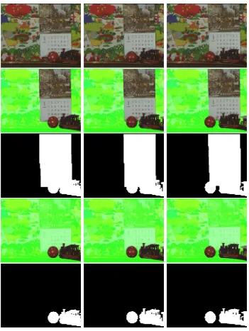
Figure 2.2: Examples of the binary alpha mattes for frames 1 (left), 12 (center) and 25 (right) in the Calendar and Mobilesequence, where these frames are shown in thetop row.

Third row: The alpha mattes considering the calendar, train and ball all constitute the foreground. The foreground extracted with these mattes are shown in the second row. Here the background is shaded in green. Bottom row: The alpha mattes considering only the train and ball constitute the foreground. The foreground extracted with these mattes are shown in the fourth row. A pixel site s coloured black or white in an alpha matte correspond to

(24)

Objects

Coherent Motion Regions

Coherent Appearance

Regions

Motion Features

Colour, Texture and Edge

Features

Video/Image Pixel Data

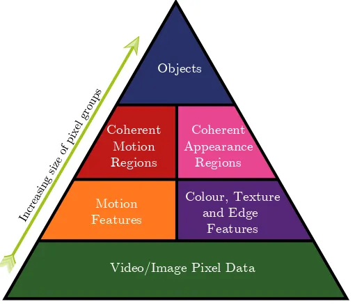
[image:24.595.174.429.110.328.2]

Increasing size of pixel groups

Figure 2.3: The heuristics used in generating video object segmentations. Motion (orange), colour, texture and edge (purple) features are extracted from the pixel data (green). These features are then utilized in finding spatially and temporally coherent motion (maroon red) and appearance (pink) regions in the images of a sequence. These coherent regions are expected to exclusively represent a single object (blue) in scene. As we move up (green arrow) this heuristic pyramid we increase the number of image pixels that are grouped together.

(center) and 25 (right) in the well knownCalendar and Mobile sequence. The third row shows the mattes where the calendar, train and ball are all considered to constitute the foreground. Also shown in the bottom row are the mattes where only the ball and the train are foreground. The second and third rows (fig. 2.2) show the foregrounds extracted with the corresponding mattes in the third and bottom rows respectively. Here the background in each image is shaded green.

2.2 A Pyramid of Techniques

Previous VO segmentation techniques generally rely on motion and appearance cues in order to generate the required segmentations. However, there are some techniques where only motion or appearance information is used exclusively [23, 127]. All previous approaches in some way generate heuristics from motion and appearance cues to facilitate the segmentation of an image sequence.

(25)

2.2. A Pyramid of Techniques 13

there are no computer vision algorithms that can reason about real scenes at this level in a useful way. Only human perception can be used to decompose a complex visual scene into objects.

The next level down from the objects in a scene (fig. 2.3) consists of spatially and temporally coherent motion (maroon red) and appearance (pink) image regions. VO segmentation tech-niques can be considered to operate at this level. These coherent regions can be identified in a sequence using a combination of motion (orange), colour, texture and edge (purple) features. These features are extracted from the raw video/image pixel data (green) at the lowest level.

All VO segmentation techniques can be considered to be estimating analpha matte αf(s) for imageIf(s), given a set of model parameters Θf(s). This task can be expressed in the Bayesian framework below, where the solution to the segmentation problem is the Maximum a posteriori (MAP) estimate of αf(s).

αf(∼s) are the labels in some defined neighbourhood of pixel sites at frame f. VO segmenta-tion techniques generally differ in how they go about determining the various models and their corresponding parameters Θf(s). These models are used to describe the coherent motion and appearance regions in fig. 2.3. With the right parameters Θf(s), these models explain the ob-served motion, colour, texture and edge features at the lower heuristics levels, which usually are part of the likelihood design. The design of the priorps(αf(s)|.) typically fulfills the requirement for the coherent regions to be spatially and temporally smooth over a sequence.

In the case where all the object in an image sequence are rigid and consistent in appear-ance and motion, there are VO segmentation techniques that will segment this sequence at the ‘objects’ level. That is, every object with unique motion and appearance can be completely extracted from these sequences. However, real world sequences of interest do not fall into this restricted category of sequences that comprise of only rigidly moving objects. Real world se-quences usually contain articulated non-rigid objects that may have inconsistent motions and appearances. There might be several coherent motion and appearance regions (fig. 2.3) associ-ated with each of these objects. A human would be required to associate these coherent regions with a particular object.

2.2.0.1 Technique Categories

The need for high quality segmentations of real world sequences has motivated a category of VO segmentation techniques that we defined as supervised techniques. Thesesupervised techniques include a user in the segmentation loop, in order to handle difficult sequences. These techniques emerged in the late 90s, where the technique proposed by Mitsunaga [76] in 1995 is an early example of a supervised VO segmentation approach.

We define a VO segmentation technique where no user assistance is utilized as anunsupervised

(26)

the in the late 70s, Adelson [3] and Thompson [110] in the early 80s. Since there is no human in the segmentation loop, these techniques produce much lower quality segmentations compared tosupervised techniques.

In supervised VO segmentation techniques the user usually interacts with the system at the ‘objects’ level (fig. 2.3). Here the user may supply reference alpha mattes for some of the frames in a sequence and then allow the system to segment the remaining frames [11, 12, 100]. In these user supplied alpha mattes the objects of interest are specified to the system. These object specifications at the ‘objects’ level in the heuristics pyramid (fig. 2.3), constrain the lower level heuristics (coherent motion and appearance regions, etc). Hence the various heuristics are constrained implicitly from the top (‘objects’) of the pyramid to the bottom (‘video/image pixel data’). These constraints allow supervised systems to discriminate better between the features (motion and appearance) of the various objects in a sequence.

Fig. 2.2 shows examples of user supplied alpha mattes for frame 1 (left), 12 (center) and 25 (right) for the Calendar and Mobile sequence. In the third row the user specifies that the foreground consists of the calendar, train and ball. However, in the bottom row the foreground consists of the ball and the train only. This user interactivity makes thesupervised system more useful in modern applications such as post production.

Unlike asupervised technique, anunsupervised technique has to gather the various heuristics from the bottom (‘video/image pixel data’) of the pyramid (fig. 2.3) to the top (‘objects’). Since theseunsupervisedsystems have no notion of what constitutes an object, there are no guarantees that the segmentations produced would be in some way useful.

2.2.0.2 Challenges of VO Segmentation Techniques

There are some fundamental issues which affect all video object segmentation techniques, irre-spective of whether they are supervised or unsupervised. Perhaps the most important is main-taining spatial and temporal consistency from frame to frame for the segmentation of an image sequence. The human visual system is very sensitive to temporal inconsistencies that may occur in an image sequence [122]. Segmenting the frames in a sequence independent of each other often results in temporal incoherencies. Hence learnt heuristics at each frame must be propagated in some way over a sequence. Typical video cameras only capture at 25 fps, thus the sampling rate is too low for dealing with the motion of fast objects and often introduces motion blurs. Hence building correspondence across frames and maintaining temporal coherence is very difficult in this case.

Another issue which affects onlysupervised techniques is how to effectively use the informa-tion supplied by the user in segmenting the sequence. Here the user may specify alpha mattes

(27)

2.3. Unsupervised Techniques 15

segmentations.

We will discuss later how the various VO segmentation techniques handle these issues.

2.3 Unsupervised Techniques

As previously mentioned,unsupervised techniques do not utilize any user supplied information. The majority of these techniques employ the idea of using ‘layers’ to represent the image regions in a sequence. Here a ‘layer’ simply refers to an image region where all the pixels have similar motion and/or appearance according to a specified model. For example, an Affine motion model may be used for specifying motion layers. ‘Layers’ correspond to the coherent motion and appearance regions in fig. 2.3 as discussed previously.

The idea of segmenting an image into layers was introduced by Wang [127] and Pentland [35, 87, 88] during the early 90s. This idea become very popular because it is an intuitive way of thinking about how images are structured.

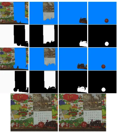
Fig. 2.4 shows examples of typical layers for frames 1 (first row) and 25 (third row) in the

Calendar and Mobile sequence. Here the pixels for the background (left), calendar (left center), train (right center) and ball (right) constitute the four layers shown respectively. The alpha mattes of the layers for frames 1 and 25 are shown in the second and fourth rows respectively.

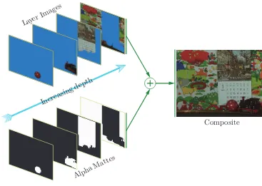
An image can be composited from a set of layers (specifically the image data) and the correspondingalpha mattesfor that image. Also the depth order of these layers must be specified. Fig. 2.5 illustrates the composition of frame 1 in the Calendar and Mobile sequence from the four layers for this frame (fig. 2.4).

2.3.1 Layer-based Techniques

With the introduction of the layer representation [35, 87, 88, 127], researchers were given a plat-form for integrating spatial and temporal smoothness strategies into the segmentation process. In the original work of Wang, optical flow [53] between adjacent frame pairs was used to extract motion layers. The use of only two frames at a time led to temporal inconsistency in the layers extracted. Also no spatial smoothness schemes were utilized in assigning pixels to the various layers. Hence there was room for improvement in this foundational work.

(28)

[image:28.595.72.527.115.629.2]

Figure 2.4: The layer representation of frames 1 (bottom left) and 25 (bottom right) in the

Calendar and Mobilesequence. Top and third rows: The layer images for the background, calendar, train and ball for frame 1 and 25 respectively. Second and fourth rows: The alpha mattes (α) for the corresponding images in the top and third rows. Here a pixel site scoloured

(29)

Increasi

ngdep

th

Alpha Mattes Layer Images

[image:29.595.128.495.106.367.2]

Composite

Figure 2.5: The composition of frame 1 in the Calendar and Mobile from the layer images and the alpha mattes. The depth ordering determines how the pixels from the various layers occlude each other.

this technique since the sprite maintains a consistent appearance throughout an image sequence. However, this technique is only effective on sequences where the motion of the objects can be approximated with parametric models.

Prior to Jojic [58], Ayer [9] and Sawhney [105] both presented techniques that also utilized EM for determining motion layers using optical flow. Smith [109] identified that these EM based approaches only work well when the motion of the objects in a sequence are very distinct. If the motions of the objects are quite close, the EM algorithm may fail to converge when estimating the layers. This non-convergence leads to the overall failure of the segmentation process. Also most of these approaches are prone to local minima, namely those described in [32, 58, 105, 116], that use EM or variational methods for learning the parameters of the layers.

Another EM based approach was proposed by Weiss [128], where a Markov Random Field [48] (MRF) model was used to encourage label smoothness in the assignment of pixel to the layers. Employing MRFs for enforcing spatial smoothness is common in a lot of approaches [34, 40, 64, 79–81]. Boykov [25, 135] provided a convenient way of finding the optimal solution to MRF problems using graphs (Graphcuts). Hence researchers [30, 56, 131] in the 2000s started formulating the layer segmentation problem in MAP-MRF frameworks which were then solved with Graphcuts.

(30)

Kumar uses a MAP-MRF framework which is solved with loopy belief propagation. Also unlike Jojic, Kumar has more tolerance for the change in motion and appearance of the layers over the duration of a sequence (flexible sprites).

Criminisi [33] proposed a real-time layer-based technique that used a Conditional Random Field (CRF) [65] and a second order Hidden Markov Model prior to enforce spatial and tem-poral smoothness respectively. CRFs play a similar role to MRFs, except they are not prone to the label bias problem [65]. Hence the use of CRFs instead of MRFs should provide better segmentations. However the results of Criminisi [33] were not significantly better than previ-ous layer-based techniques. This was probably because Criminisi’s approach had a real-time constraint, where future frames are not available for the current segmentation.

2.3.1.1 Two Layers

Determining the optimal number of layers for a sequence is a challenging task. Hence some techniques simply assume a two layer representation [16,34,62,82]. Here one layer represent the background, and all other objects are assigned to the other layer (foreground). The motion of the background layer is assumed to be the estimated global motion. All pixels which do not follow the motion of the background, are assigned to the foreground layer.

The two layer technique by Kokaram [62] in 2005 is typical of these two layer approaches. It has been implemented in a software package calledNUKE developed by The Foundry [2]. The algorithm is included in the MotionMatte plugin bundled into version 4.7 and all subsequent versions of NUKE. We will use this technique as a baseline to compare performance later.

Kokaram [62] presented a Bayesian framework where the likelihood design was based on motion compensated displaced frame differences (DFDs) for the current frame with respect to multiple past and future frames. The corresponding past and future frames were motion compensated with respect to the motion of the background layer. The motion of this layer was assumed to be the global motion, and this motion was estimated with a technique in [63] which disregards the motion of the foreground. The likelihood design here constrains the alpha value

αf(s) for pixel site s at frame f to be 1 (foreground) when the motion compensated DFDs for this site are large in both future and past temporal directions. Spatial smoothness was injected via an MRF prior. The MAP estimates for the binaryalpha mattes were then generated using the Iterated Conditional Modes (ICM) algorithm [17].

2.3.2 Region Merging and Hierarchical Clustering Techniques

(31)

To overcome the errors at the boundaries of motion layers inherited from the use of optical flow, some researchers have proposed other unsupervised techniques. Some of these techniques can be placed into two categories, which we define asregion merging and hierarchical clustering

techniques.

Region merging approaches [4, 39, 78] generally perform two separate motion and colour segmentation [28] processes. It is assumed that the colour segments are almost always a subset of motion segments. That is, the majority of the pixels in a colour segment usually correspond to one motion segment. Unlike the boundaries between motion segments, the boundaries between the colour segments are assumed to be more closely related to the actual object boundaries in an image. Hence the colour segments are combined in a strategic way using the motion segments as guides. These combined colour segments represent the final segmentation, in which the boundaries of the objects are better defined compared to those in the motion segmentation result.

Obviously region merging techniques fail when the foreground and background colours are similar, since the colour segments would extend across both the foreground and background image regions. There is also a dependence in these techniques on the quality of the motion segmentation step. Here a poor motion segmentation will lead to a poor final segmentation.

2.3.2.1 Hierarchical Clustering

Hierarchical clustering techniques [50, 85, 86] treat an image sequence as a 3D spatiotemporal volume [61], and typically use a variant of the Mean shift algorithm [28] for segmentation [37, 126] based on colour only. These techniques started to emerged in the early 2000s, with the improvement in the amount of computational resources available in standard computers. These approaches require a significant amount of memory since all the video data usually need to be manipulated at once.

The approach presented by Grundmann [50] in 2010 is a typical example of a hierarchical clustering technique. Grundmann [50] extended an image segmentation technique by Felzen-szwalb [41] to handle the segmentation of videos. In the work of FelzenFelzen-szwalb [41] an image is segmented by using a graph-based clustering technique. The pixels in an image are the nodes in a derived graph structure. In this graph each pixel site is connected to its 8 immediate neighbours via edges. Edge weights are derived from per-pixel normalized colour differences. Subsequently, pixels are merged into image regions by traversing the edges and evaluating whether the edge weights are smaller than some estimated local thresholds. These thresholds are generated ac-cording to local image texture. The final set of image regions constitute the segmentation.

(32)

[image:32.595.112.485.101.331.2]

Figure 2.6: Segmentation results taken the paper by Grundmann [50]. Shown are two frames from four sequences with their corresponding segmentations. The coherent appearance regions are coloured in a similar ways for the segmentations of each sequence. For example, the face of the actor in the bottom row is coloured orange in both segmentations. Top and second rows: A sequence of a water-skier and an America football game respectively. Third row: A sequence from the movie Public Enemies, © 2009 Universal Pictures. Bottom row: A sequence from the movie No Country for Old Men,© 2007 Miramax Films.

thresholds for merging are varied to produce a tree of various segmentation levels. Here small conservative thresholds over segment the sequence, while large thresholds have the opposite ef-fect. Therefore as we move down this tree the sequence become more segmented (over segmented at the lowest level). The idea is that the user can then select the level of segmentation required from those in the generated segmentation tree.

The implementation of Grundmann [50] is quite sophisticated in order to work around com-putational memory issues. Fig. 2.6 shows the segmentations reported by Grundmann [50] on four image sequences. Note here that only the segmentations at a selected level in the segmentation tree are shown. From these segmentations it may be observed that the technique of Grundmann does not provide good segmentation for some of the boundaries between the objects in these four sequences. This technique is mainly dependent on appearance (colour) information, hence it suffers from not utilizing motion information in a useful way.

(33)

2.4. Supervised Techniques 21

2.4 Supervised Techniques

As previously defined asupervised VO segmentation technique utilizes user supplied information in order to generate high quality segmentations. The user may supply for some frames in a sequence partially labelledmattes calledtrimaps, or fully segmented binaryalpha mattes, which we define askey frames. Also the user may just supply a few foreground and background paint strokes on selected frames.

In atrimap, image regions of definite foreground (αf(s) = 1) and background (αf(s) = 0) are labelled along with unknown regions (αf(s) = ?). The segmentation system is subsequently required to generatealphavalues for the pixels in these unknown region (αf(s)∈[0,1]), thus pro-ducing a continuousalpha matte. Note that binary and continuousalpha mattes are sometimes referred to as ‘hard’ and ‘soft’alpha mattes respectively in the literature. Also VO segmentation techniques produce ‘soft’alpha mattesfor the frames in a sequence are calledvideo matting tech-niques. For the rest of this discussion it should be assumed that all VO segmentation techniques mentioned produce binary (‘hard’) alpha mattes unless we specify otherwise.

2.4.1 Adaptation of Image Segmentation Techniques

Some supervised VO segmentation techniques [10, 27, 52] to date are simply adaptations of successful interactive image (supervised) segmentation techniques [24, 66, 71, 102, 103, 134] to the problem of segmenting video sequences. Wang and Cohen [125] provide a comprehensive review of these interactive image segmentation approaches.

Operating on each individual frame of a video independently using only an interactive image segmentation (IIS) technique would create some undesired problems. These IIS techniques [21, 26, 67, 71, 102, 103, 124, 134] usually require that the user supplies for an image a trimap or paint foreground and background strokes. Doing this for every frame in a video would be a tedious task. An additional problem is that slight differences in the extraction of the foreground from frame to frame would lead to obvious temporal inconsistencies, especially along the edges of the foreground.

Unlike still image segmentation techniques, VO segmentation techniques can exploit motion information. Each video frame is temporally correlated with the nearby frames. Hence the challenge forsupervised VO segmentation techniques is to accurately identify foreground regions with minimal user assistance by utilizing all available motion and appearance information.

Chuang et al. [27] in 2002 proposed a video matting technique based on a Bayesian image matting technique [134] they presented earlier. In this technique [27] optical flow was used to propagate a set of user drawn trimap to the unspecified frames in a sequence. A clean background plate was estimated as well to assist in the segmentation process. With a trimap

(34)

the optical flow estimation, which is often quite erroneous. Furthermore, the background plate estimation assumes the background undergoes only planar-perspective transformation, which is not true of most real world sequences of interest. This technique would fail if the objects in the background are moving.

2.4.2 Propagation of Binary Mattes

A subcategory of supervised VO segmentation techniques [11, 12, 70, 100, 123] require the user to supply fully segmented binary alpha mattes (key frames) for selected frames in a sequence. The segmentation system then automatically produces binary alpha mattes for the remaining frames in the sequence by propagating the labels in these key frame in some way. The binary

alpha mattes are then generally used to automatically generate trimaps for each frame in a sequence. Once these trimaps are estimated, an image matting technique can then be used to create continuous (‘soft’) alpha mattes. These VO segmentation techniques [11, 12, 70, 100, 123] reduces the work load of the user, astrimapsdo not have to be specified manually for every frame in a sequence. Hence less user interactions are required compared to the previously discussed approaches that are adaptations of image segmentation techniques.

Liet al.[70] in 2005 extended the pixel-level 3D Graph cut technique proposed by Boykov [26] to better handle video sequences. They use three main steps in their technique, which are a 3D Graph cut binary segmentation, tracking user defined local image windows for correcting the binary segmentation, and extracting continuous alpha mattes with an image matting technique [107]. The first two steps are used to produce accurate binaryalpha mattes, from whichtrimaps

are generated for the final image matting step. The user initially supplies fully segmented binary

key frames for some of the frames in a sequence. These key frames are articulated in the 3D Graph cut segmentation step, and the user then corrects any undesired segmentation errors.

In the next two sections we will discuss the Video SnapCut [12] and Feature-Cut [100] techniques, as we compare our work to both techniques later in this thesis. Both techniques proposed in 2009 are state of the artunsupervised VO segmentation techniques which propagate user defined binaryalpha mattes.

2.4.2.1 Video SnapCut

TheVideo SnapCutsegmentation algorithm was proposed by Baiet al.[12]. An implementation of this algorithm is bundled into Adobe After Effects CS5 [1] as a matting tool called Roto Brush.

This algorithm uses local motion information to propagate appearance information from a segmented frame t to the current unsegmented frame t+ 1. This appearance information is captured in overlapping rectangular windows of fixed sizes placed along the contour of the foreground. These local windows are defined aslocal classifiers in the paper [12]. The top row

of fig. 2.7 shows examples of these local classifiers Wt

(35)

[image:35.595.153.481.99.405.2]

2.4. Supervised Techniques 23

Figure 2.7: This figure is taken from the paper by Bai et al. [12] which is an illustration of the local classifiers proposed in the paper. (a): Overlapping classifiers (yellow squares) are initialized at frame t along the contour of the foreground (red curve). (b): These classifiers are then propagated onto the next frame using local motion information. (c): Each classifier contains a local colour and shape model, which are initialized at frametand refined if necessary at frame t+ 1. (d): Local foreground/background classification results are then combined to generate a global likelihood for all the pixels in frame t+ 1. (e): The final segmentation for frame t+ 1. Video courtesy of Artbeats.

Wt

kin frame t(left) and propagated to the current framet+ 1 (right) using motion information obtained from optical flow [53] and SIFT [73] feature matching. Here the local classifiers W_kt

(window) in frametcorrespond toW_kt+1 in framet+ 1. In eachlocal classifier colour and shape models (middle row of fig. 2.7) are generated for the foreground/background image region inside the corresponding window. These models are then used in the design of a posterior distribution for the alpha labels for the current frame t+ 1. Finally, a MAP estimate for the binary alpha matte for this framet+1 is generated using a Graph cut [135] solution. Thebottom row of fig. 2.7 shows an example of the likelihood probability map on the left (d) for the frame segmented on the right (e).

(36)

[image:36.595.138.454.98.312.2]

Figure 2.8: This figure is taken from the paper [100] by Ring. This is an example of propagating a user define alpha matte for frame 1 to the an unsegmented 5th frame in a sequence of a Polo player. Using feature correspondences (green lines) between these frames, regions of the known matte at frame 1 are ‘pushed’ into frame 5. Each of the blueand red circles represent the neighbourhoods of the respective SIFT features that have been matched in both frames. The partial matte in frame 5 is missing some foreground regions, but the subsequent optimization process (MAP estimation for labels) usually is able to fill in these missing region.

key frame) in a sequence, and all subsequent frames are processed in the order 2 toT (whereT

is the number of frames in the sequence). The user is allowed to correct any segmentation errors generated for the current frame t+ 1, and by default these changes only affect the frames after

t+ 1 (forward propagation), i.e. frames t+ 2, . . . , T. However the user can make the current frame t+ 1 a key frame, and allow previous frames (2 to t) to be influenced by this key frame

(backward propagation).

It will be shown later in this thesis that this technique generally performs well. However, it has some issues with distinguishing revealed background regions from legitimate foreground regions.

2.4.2.2 Feature-Cut

(37)

2.5. Sparse Video Object Segmentation 25

frames from a sequence of a Polo player. Here the user supplies a binary alpha matte for frame 1 (left), and this mattes is ‘pushed’ into the unsegmented 5th frame (right). At each pixel sites in the unsegmented framef, votes are accumulated whether sites is foreground or background. These votes are accumulated from all the user suppliedalpha mattes within a temporal window of the the current unsegmented framef. These foreground/background votes for each pixel site are utilized in the design of a likelihood distribution. Ring then proceeds to generate a MAP estimate of the binary alpha matte for frame f, using a Graph cut solution, and a MRF prior distribution.

This technique does not utilize appearance information in the traditional sense of colour and/or shape modelling. The author use the intensity of matched pixels in SIFT neighbourhoods to influence the foreground/background votes. Hence, this technique has some issues with the temporal consistency of the segmentations produced from frame to frame. Also for image sequences with low texture there are usually not enough SIFT feature matches between the frames for effective matte propagations. Therefore poor segmentations are usually produced for sequences with relatively low image texture.

2.5 Sparse Video Object Segmentation

The techniques discussed previously produce a label for every pixel in a sequence. We define these techniques as producing adense segmentation. However, there is another category of video object segmentation techniques that only label a sparse set of pixel sites in a sequence. We define these techniques as producing a sparse segmentation. In general, these sparse segmentation techniques utilize feature point trajectories such as Kanade-Lucas-Tomasi (KLT) tracks [55] for estimating the various coherent regions (layers) in a sequence. Hence these techniques explicitly use only motion information.

Fig. 2.9 shows examples of dense (center) and sparse (right) segmentations for frame 5 in the Calendar and Mobile sequence. The spatial locations of the trajectories at frame 5 are in-dicated with coloured ‘dots’ in thesparse segmentation on the right. The motion history of the trajectories are indicated with lines that extend from the corresponding ‘dots’. Both segmenta-tions (dense and sparse) were produced with unsupervised techniques we will propose later in this thesis. The dense segmentation is estimated from the sparse segmentation by associating in some way the pixels in a sequence with the various trajectory groups (bundles). The corre-sponding sparse and dense image regions are coloured in a similar way in both segmentations. For example the pixels and trajectories for the calendar are coloured yellow in the dense and

sparse segmentations respectively.

(38)

Figure 2.9: Examples of thedense(center) and sparse(right) segmentations of frame 5 (left) in theCalendar and Mobilesequence. Thedensesegmentation is produced using thesparse

segmentation in a technique we will propose later in this thesis. Corresponding sparse and dense segmentation regions are coloured in a similar way. Right: Thesparsesegmentation for frame 5, where the spatial location of the trajectories are indicated with coloureddots. The line that extends from each dots show the motion history of the corresponding trajectory.

a sparse segmentation for ‘guiding’ this dense segmentation process. Here the objects in the finaldense segmentation were of a reasonable quality compared to other equivalent unsupervised VO segmentations techniques. Wills et al. [129] were the first to propose this two step idea, where a sparse and then a dense segmentation is performed.

For the technique of Wills et al. [129], the motion layers were estimated in the sparse seg-mentation step, and subsequently the pixels in a sequence were assigned to these layers in the finaldense segmentation step. Feature point trajectories are generated for thesparse segmenta-tion step by matching F¨orstner interest points [45] across adjacent frames in a sequence. These trajectories were then clustered using a variant RANSAC algorithm [42], where each cluster represents a specific motion layer. The motion models for the layers were proven to be more reliable than those obtained with a technique that uses a dense optical flow field instead of sparse point trajectories. This idea was supported by Xiao [56] in 2005, who presented a similar two step (sparse then dense) approach.

2.5.1 Categories for Sparse Techniques

(39)

Figure 2.10: Left: A truck shown at frames 1 in a motion sequence from the Hopkins dataset [117] available online. Some roughly planar surfaces on the truck are highlighted in red, green, yellow, purple, and cyan. Center: The desired labels for a 3D segmentation technique. The points along the trajectories for the background and truck areredandyellowdots respectively.

Right: The trajectory segmentation result produced by our proposed sparse segmentation technique. Each trajectory bundle shown in a different colour roughly represents a single surface of the truck.

A sparse 3D segmentation technique can be considered to group trajectories of similar 3D motion. However, a 2D sparse segmentation technique groups trajectories of coherent 2D mo-tion in the image plane, according to a defined momo-tion model (e.g. Affine). The number of 2D trajectory groups for a sequence may not correspond to the number of 3D objects. The illus-tration on the right of fig. 2.10 shows the 2D segmentation for the ‘truck’ sequence produced by a technique we will propose later in this thesis. Here each of the 10 trajectory group labels is indicated with a different colour. The perspective of the scene with respect to the camera causes different image regions to have varying 2D motion in the image plane. For example the front of the truck moves faster than the side in the image plane.

2.5.2 Sparse 2D Segmentation Techniques

As previously mentioned, sparse 2D segmentation techniques group feature point trajectories with coherent 2D motion in the image plane according to a specified motion model. The sparse

segmentation performed by Wills [129, 130] discussed previously is the earliest example of these techniques. Even though there were earlier techniques that segment feature point trajectories in some way, we are only interested in techniques that are in some way applicable to the dense

segmentation problem. Therefore we will only discuss techniques that fit this criterion.

(40)

2.5.2.1 Affine Region Growing

The approach proposed by Pundlik groups KLT [55] trajectories with coherent motion according to Affine motion models. We define each group of trajectories with coherent motion as a trajec-tory bundle. Each trajectory bundle represents a single motion layer. The segmentation system of Pundlik is causal, therefore in his design the segmentation for the current frame depends only on the trajectories that exist for the current framef, and the previous framef ₋1.

Let there be T trajectories _Xt, t∈ {1 : T}, whereXt is a trajectory that exist at both the current and previous frames at the minimum. Pundlik determines the neighbourhood structure for these spare trajectories_Xt by performing Delaunay triangulations on the spatial locations of these trajectories at the previous framef−1. A trajectory bundle ( motion layer) is discovered by first selecting a trajectory at random and examining if its motion is similar to the motion of its neighbouring trajectories. This trajectory and its neighbours are grouped together if the defined error for each trajectory using the Affine motion model is below a threshold. The group is then allowed to expand until no more neighbouring trajectories can be placed in the group. When the first group/bundle is completely discovered, another ungrouped trajectory Xt is selected at random, and the process is repeated to discover the other bundles.

At every framef ∈ {2 :F}trajectory bundles are discovered in the manner described above, whereF is the number of frames in a sequence. Pundlik tries to assign any new trajectories at framef to the bundles previously discovered in framef₋1 if this is possible, else new bundles are formed. This ad hoc method of identifying trajectory bundles leads to temporal inconsistencies in the motion layers discovered. Also just using motion information over two adjacent frame f

and f −1 at a time does not allow this technique to discriminate well between the motions of the various trajectory bundles (motion layers).

2.5.2.2 J-Linkage

Fradet [46] proposed a technique where Affine motion models were estimated for a sequence using the J-Linkage algorithm [112]. The J-Linkage algorithm presented by Toldo [112] in 2008 is a model fitting algorithm similar to RANSAC [42], where the aim is to identify a set of models that describe some given noisy data that may contain outliers.

Using the J-Linkage algorithm a set of random Affine motion models are generated from the trajectories (KLT [55] trajectories are used for most sequences) with the longest duration in a sequence. The models that best explain the observed trajectory data are kept. Each model kept describes the motion of a particular trajectory bundle. Hence a trajectory Xt is assigned to bundle nif the corresponding motion for bundlen describes the motion of trajectory_Xt the best out of all the bundles.

(41)

with short durations are not described well. These short trajectories usually correspond to non-rigid objects. Hence, this technique may not provide motion layers that describe non-non-rigid motions in a useful way.

2.5.3 Sparse 3D Segmentation Techniques

Sparse 3D segmentation techniques [59,97,119,132] group trajectories with coherent 3D motion. In general these techniques derive a motion feature space by factorizing (usually with SVD) a matrix formed from the spatial locations of the trajectories in a sequence. The idea is that trajectories that have similar 3D motion reside in a low dimensional subspace in this derived feature space. Hence the solution to the segmentation problem is locating each subspace cor-responding to an independently moving 3D object. To locate these subspaces, a clustering or polynomial fitting technique is usually applied to the trajectory points in the derived feature space. Tron [117] provides a comprehensive review of these techniques.

These 3D segmentation techniques have limited applications, since they work only for se-quences with rigidly moving objects. Also the quality of the segmentations produced by these techniques deteriorate as the number of objects with different motions increases in a sequence. To date, the state-of-the-art 3D segmentation techniques can successfully segment sequences with a maximum of three independently moving objects. Another issue with these techniques is that the number of objects in the sequence most be specified by a user.

2.5.4 Spatial Inference from Sparse Segmentations

It seems sensible that doing a sparse trajectory segmentation should be a powerful step in a subsequent dense pixel segmentation of an image sequence. In 2008 we began to explore this idea for a visual surveillance application [15] where inaccurate foreground delineation was tolerable. We only wanted to detect if a new object had been introduced in an outdoor scene of interest. Fig. 2.11 shows two sequences;Dumping Pedestrian (687 frames) andDumping Car

(1099 frames) which are typical examples of the type of sequences we are interested in for this surveillance application. In both sequences black garbage bags are placed into the respective scenes. We are able to detect the presence of these new objects from the segmentations performed by our technique.

(42)

Figure 2.11: Example sequences our surveillance application is expected to segment. Top row: Frames 1, 321 and 613 in theDumping Pedestriansequence of 687 frames. In this sequence a pedestrian enters and exits the scene leaving a black garbage bag behind. Bottom row: Frames 1, 545 and 1097 in the Dumping Car sequence of 1099 frames. In this sequence a car enters and exits the scene leaving a small black garbage bag behind.

matching features in the background model. The top row shows the corresponding frames for the feature maps in the second row. Note that there are features classified as foreground that actually correspond to background objects. These features are generated due to environmental changes subsequent to the background modelling step. Hence these features are not included in the background model. However, we design a foreground pseudo-likelihood map which helps to identify legitimate foreground features from these new background features generated due to environmental changes.

The pseudo-likelihood map generated for framef considers the spatial locations of the fore-ground and backfore-ground features. The idea is that an image region is more likely to be forefore-ground if it has a high density of foreground features. Also this image region must have a low density of background features as well. The foreground and background features are superimposed on these foreground pseudo-likelihood maps in thesecond row of fig. 2.12. Here high and low foreground likelihood values are coloured inbright orange andblack respectively.

2.5.4.1 Tracking Foreground Regions

(43)

τ

= 229

τ

= 256

τ

= 61

τ

= 226

τ

= 124

Figure 2.12: Top row: Frames 283 (left), 529 (center) and 278 (right) in theDumping Pedes-triansequence. Second row: Foreground (×) and background (.) feature points superimposed on a foreground pseudo-likelihood map, for the frames in the top row. In this pseudo-likelihood map high and low foreground likelihoods are coloured bright orange and black respectively.