A Block Procedure with Linear Multi Step Methods Using Legendre Polynomials for Solving ODEs

http://dx.doi.org/10.4236/am.2015.64067

A Block Procedure with Linear Multi-Step

Methods Using Legendre Polynomials for

Solving ODEs

Khadijah M. Abualnaja

Department of Mathematics and Statistics, College of Science, Taif University, Taif, Saudi Arabia Email: [email protected]

Received 11 March 2015; accepted 26 April 2015; published 29 April 2015

Copyright © 2015 by author and Scientific Research Publishing Inc.

This work is licensed under the Creative Commons Attribution International License (CC BY).

http://creativecommons.org/licenses/by/4.0/

Abstract

In this article, we derive a block procedure for some K-step linear multi-step methods (for K = 1, 2 and 3), using Legendre polynomials as the basis functions. We give discrete methods used in block and implement it for solving the non-stiff initial value problems, being the continuous interpolant derived and collocated at grid and off-grid points. Numerical examples of ordinary differential equations (ODEs) are solved using the proposed methods to show the validity and the accuracy of the introduced algorithms. A comparison with fourth-order Runge-Kutta method is given. The ob-tained numerical results reveal that the proposed method is efficient.

Keywords

Collocation Methods with Legendre Polynomials, Initial Value Problems, Perturbation Function, Fourth-Order Runge-Kutta Method

1. Introduction

a system of differential-algebraic equations.

In this paper, we present an efficient numerical method to solve numerically the ODEs. The proposed method is a block procedure for some K-step linear multi-step methods (for K = 1, 2 and 3) [17] using Legendre poly-nomials as the basis functions. In addition, we give discrete methods used in block and implement it for solving the non-stiff IVPs that were the continuous interpolant derived and collocated at grid and off-grid points. In this article, we consider the general form of the first order initial value problem

( )

(

,

( )

)

,

( )

0 0

y x′ = f x y x y x =y . (1)

The plan of the paper is as follows: In Section 2, the derivation of the proposed methods is presented. In Sec-tion 3, stability and convergence analysis of the block schemes is given. In SecSec-tion 4, two numerical examples are considered. The paper ends with summary and conclusions in Section 5.

2. The Derivation of the Proposed Methods

In this section, we derive discrete methods to solve (1) at a sequence of nodal points x_n =x₀+nh where h>0

is the step-length or grid-size defined by h=x_n+₁−x_n and y x

( )

denotes the true solution to (1) while the ap-proximate solution is denoted by y x

( ) {

= y yn, n+₁,,yN

}

, for some positive number N. The proposed method depends on the perturbed collocation method with respect to the power series method is used as the basis for collocation approximation with the Legendre polynomials as the perturbation term.

In the first we consider the approximate solution of the perturbed form of (1) in the following power series [18]-[21]

( )

( )

0

,

K

K i i n n K

i

y x c

ψ

x x x x+

=

=

∑

≤ ≤ . (2)

where

( )

i, 0,1, ,

i x x i K

ψ

= = _ . (3)

Substituting from Equation (2) in Equation (1) we have

( )

( )

( )

1

,

K

i i K

i

c

ψ

x f x y

λ

L x =

′ = +

∑

, (4)

where L_K

( )

x is the Legendre polynomial of degree K, valid in x_n≤ ≤x x_{n K}+ and

λ

is a perturbed parame-ter. In particular, we shall be dealing with cases K = 1, 2 and 3 in (2) and (3).

The well-known Legendre polynomials are defined on the interval

[

−1,1

]

and can be determined with the aid of the following recurrence formula [22] [23]

( )

( )

( )

1 1

2 1

, 1, 2,

1 1

i i i

i i

L x x L x L x i

i i

+ −

+

= − =

+ + ,

where the first four polynomials are

( )

( )

( )

(

2

)

( )

(

3

)

0 1 2 3

1 1

1, , 3 1 , 5 3

2 2

L x = L x =x L x = x − L x = x − x . (5)

In order to use these polynomials on the interval

[

x xn, n K+

]

we define the so called shifted Legendre poly-nomials by introducing the change of variable

(

)

(

)

2

, 1, 2, 3

n K n

n K n

x x x

x K

x x

+

+

− +

= =

− . (6)

Cases Study

Case 1: If K = 1

( )

1 1

1

2

1,

n n n

n

n n

x x x

L x x x + + − − = = − −

(

)

1 1

1 1

1

2

1

n n n

n

n n

x x x

L x x x + + + + − − = = − .

In addition, from Equation (3) we can deduce that ψ ′₀

( )

x =0, ψ ′₁

( )

x =1. Then, the Equation (4) will reduce to the following form

( )

( )

1 , 1

c = f x y +λL x . (7)

We now collocate Equation (7) at x_{n i}+ , i=0,1 and interpolate (2) at x=xn, we get a system of three Equations with c ii

(

=0,1

)

and parameter

λ

0 1 1 1 1 , , . n n n n c c x y

c f c f λ λ ₊ + = + = − = (8)

Using a suitable method to solve the above system to obtain

(

1

)

1 0

(

)

1

, ,

2 fn fn c fn c yn xn fn

λ= − + = −λ = − −λ

From (2), we have

( )

0 1

y x =c +c x. (9)

Now, the required numerical scheme of the proposed method will be obtained if we collocate the above Equation (9) at x=x_n+₁ and substitute c0, c1,

λ

as follows

(

)

1 1

2

n n n n

h

y+ =y + f + + f . (10)

Which is the well-known trapezoidal rule.

Case 2: If K = 2

In this case, we take the polynomial ₂

( )

1

(

3 2 1

)

2

L x = x − and use (6), then collocating this equation at x_n,

1 n

x+ and xn+2, we obtain

( )

(

)

(

)

2 2 1 2 2

1

1, , 1.

2

n n n

L x = L x+ = − L x+ =

In addition, from Equation (3) we can deduce that ψ ′₀

( )

x =0, ψ ′₁

( )

x =1, ψ ′₂

( )

x =2x. Then, the Equation (4) will reduce to the following form

( )

( )

1 2 2 , 2

c + xc = f x y +λL x . (11)

We now collocate Equation (11) at x_{n i}+ , i=0,1, 2 and interpolate (2) at x=xn, we get a system of four equations with c i_i

(

=0,1, 2

)

and parameter

λ

2 0 1 2

1 2

1 1 2 1

1 2 2 2

, 2 , 1 2 , 2 2 .

n n n

n n

n n

n n

c c x c x y

c x c f

c x c f

c x c f

λ λ λ + + + + + + = + = + + = − + = + (12)

(

)

(

)

(

)

(

)

(

)

(

)

1 2

2 2

1 1 2 2

2

0 1 2 2

1

2 ,

3 1

, 4

1 1

2 2 ,

3 2

1 1

2 2 .

3 4

n n n

n n

n n n n n n

n n n n n n n n

f f f

c f f

h

c f f f x f f

h

c y x f f f x f f

h

λ _{+ +}

+

+ + +

+ + +

= − −

= −

= + − + −

= − + − + −

From (2), we have

( )

2

0 1 2

y x = +c c x c x+ . (13)

Now, the required numerical scheme of the proposed method will be obtained if we collocate the above Equation (13) at x=x_n+₁ and substitute c0, , , c c1 2 λ as follows

(

)

1 5 8 1 11 2

12

n n n n n

h

y+ =y + f + f + + f + . (14)

Case 3: If K = 3

For case K = 3, we collocate the continuous scheme

( )

2 3

0 1 2 3

y x =c +c x c x+ +c x , (15)

at grid and off-grid points x=xn, , x=xn+₁ x=xn+₂ and x=xn+3 and this gives the required block schemes

(

)

1 39 107 1 54 2 7 3

98

n n n n n n

h

y₊ = y + f + f ₊ + f ₊ − f ₊ . (16)

3. Stability and Convergence Analysis of the Block Schemes

In this section, we present a summary on the order, the error constant and the convergence of the proposed block schemes. This summary in given in the following table.

Step K = 1 K = 2 K = 3

Order 2 2 4

Error Constant 1 12

− 1

12

− 1

96

Convergence convergent convergent convergent

4. Numerical Examples

In this section, we implement the proposed method with K = 2 and K = 3 to solve two first order initial value problems, and compare the obtained numerical results with those obtained from using the fourth-order Runge- Kutta method (RK4).

Example 1.

Consider the following IVP

( )

( )

, 0.1,

( )

0 1

y x′ = −y x h= y = .

With the exact solution y x

( )

=e−x.

The numerical results of this example are presented inTable 1 andTable 2 with the cases K = 2 and K = 3, respectively. In these tables, we presented a comparison the obtained numerical results using the proposed me-thod with the exact solution and those numerical results obtained from using RK4.

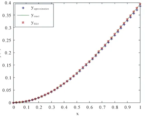
Example 2.

( )

(

1

)

, 0.1,

( )

0 0

y x′ =x −y h= y =

With the exact solution y x

( )

= −1 e−x22.

[image:5.595.145.484.191.317.2]

The numerical results of this example are presented inFigure 1 andFigure 2 with the cases K = 2 and K = 3, respectively. In these figures, we presented a comparison the obtained numerical results using the proposed me-thod with the exact solution and those numerical results obtained from using RK4.

Table 1. A comparison the proposed method at K = 2 with the exact solution and RK4: Ex-ample 1.

x Block Scheme K = 2 Exact Solution RK4

0.0 1.000000 1.000000 1.000000

0.2 0.818712 0.818730 0.818781

0.4 0.670345 0.670320 0.670541

0.6 0.548848 0.548811 0.548848

0.8 0.449215 0.449328 0.449345

[image:5.595.141.486.345.697.2]

1.0 0.367822 0.367879 0.367836

Table 2. A comparison the proposed method at K = 3 with the exact solution and RK4: Ex-ample 1.

x Block Scheme K = 3 Exact Solution RK4

0.0 1.000000 1.000000 1.000000

0.2 0.818735 0.818730 0.818738

0.4 0.670328 0.670320 0.670321

0.6 0.548817 0.548811 0.548813

0.8 0.449322 0.449328 0.449325

1.0 0.367871 0.367879 0.367873

[image:6.595.194.448.84.285.2]

Figure 2. A comparison the proposed method at K = 3 with the exact solution and RK4: Example 2.

5. Summary and Conclusions

In this paper, we presented three new block-schemes (K = 1, K = 2 and K = 3) that are convergent and absolutely stable. We used the proposed method to solve numerically a wide-range of linear initial value problems. The re-sults of the presented examples show that our method was capable for solving such problems of IVPs and gene-rates the convergence analysis, and closed to their exact solutions. This method is very simple and effective for a wide-range of ODEs. All computations are made by Matlab.

Acknowledgements

We thank the Editor and the referee for their comments.

References

[1] Hairer, E. and Wanner, G. (1991) Solving Ordinary Differential Equations II: Stiff and Differential-Algebraic Prob-lems. Springer, Berlin. http://dx.doi.org/10.1007/978-3-662-09947-6

[2] Atkinson, K.E. (1889) An Introduction to Numerical Analysis. 2nd Edition, John Wiley and Sons, New York. [3] Khader, M.M. (2013) Numerical Treatment for Solving the Perturbed Fractional PDEs Using Hybrid Techniques.

Journal of Computational Physics, 250, 565-573. http://dx.doi.org/10.1016/j.jcp.2013.05.032

[4] Khader, M.M. (2011) On the Numerical Solutions for the Fractional Diffusion Equation. Communications in Nonlinear Science and Numerical Simulations, 16, 2535-2542. http://dx.doi.org/10.1016/j.cnsns.2010.09.007

[5] Khader, M.M. (2013) The Use of Generalized Laguerre Polynomials in Spectral Methods for Fractional-Order Delay Differential Equations. Journal of Computational and Nonlinear Dynamics, 8, Article ID: 041018.

[6] Khader, M.M. (2013) An Efficient Approximate Method for Solving Linear Fractional Klein-Gordon Equation Based on the Generalized Laguerre Polynomials. International Journal of Computer Mathematics, 90, 1853-1864.

http://dx.doi.org/10.1080/00207160.2013.764994

[7] Khader, M.M. and Sweilam, N.H. (2013) On the Approximate Solutions for System of Fractional Integro-Differential Equations Using Chebyshev Pseudo-Spectral Method. Applied Mathematical Modelling, 37, 9819-9828.

http://dx.doi.org/10.1016/j.apm.2013.06.010

[8] Khader, M.M. and Hendy, A.S. (2013) A Numerical Technique for Solving Fractional Variational Problems. Mathe-matical Methods in Applied Sciences, 36, 1281-1289. http://dx.doi.org/10.1002/mma.2681

[9] Khader, M.M. and Babatin, M.M. (2013) On Approximate Solutions for Fractional Logistic Differential Equation.

Mathematical Problems in Engineering, 2013, Article ID: 391901.

In-formation Science, 7, 2011-2018. http://dx.doi.org/10.12785/amis/070541

[11] Lambert, J.D. (1991) Numerical Methods for ODE. John Wiley and Sons, New York.

[12] Sweilam, N.H. and Khader, M.M. (2010) A Chebyshev Pseudo-Spectral Method for Solving Fractional Integro-Differential Equations. ANZIAM Journal, 51, 464-475. http://dx.doi.org/10.1017/S1446181110000830

[13] Sweilam, N.H., Khader, M.M. and Nagy, A.M. (2011) Numerical Solution of Two-Sided Space-Fractional Wave Equ-ation Using Finite Difference Method. Journal of Computational and Applied Mathematics, 235, 2832-2841. http://dx.doi.org/10.1016/j.cam.2010.12.002

[14] Sweilam, N.H., Khader, M.M. and Kota, W.Y. (2013) Numerical and Analytical Study for Fourth-Order Inte-gro-Differential Equations Using a Pseudo-Spectral Method. Mathematical Problems in Engineering, 2013, Article ID: 434753, 7 pages.

[15] Hirayama, H. (2000) Arbitrary Order and A-Stable Numerical Method for Solving Algebraic Ordinary Differential Equation by Power Series. 2nd International Conference on Mathematics and Computers in Physics, Vouliagmeni, Athens, 9-16 July 2000, 1-6.

[16] Çelik, E. and Bayram, M. (2003) On the Numerical Solution of Differential-Algebraic Equations by Padé Series. Ap-plied Mathematics and Computation, 137, 151-160. http://dx.doi.org/10.1016/S0096-3003(02)00093-0

[17] Onumanyi, P., Awoyemi, D.O., Jator, S.N. and Sirisena, U.W. (1994) New Linear Multistep Methods with Continuous Coefficients for First Order Initial Value Problems. Journal of the Nigerian Mathematical Society, 13, 7-51.

[18] Fatokun, J.O., Onumanyi, P. and Sirisena, U. (1999) A Multistep Collocation Based on Exponential Basis for Stiff Ini-tial Value Problems. Nigerian Journal of Mathematics and Applications, 12, 207-223.

[19] Fatokun, J.O., Aimufua, G.I.O. and Ajibola, I.K.O. (2010) An Efficient Direct Collocation Method for the Integration of General Second Order Initial Value Problem. Journal of Institute of Mathematics & Computer Sciences, 21, 327- 337.

[20] Fatunla, S.O. (1998) Numerical Method for Initial Value Problems in ODEs. Academic Press Inc., New York.

[21] Funaro, D. (1992) Polynomial Approximation of Differential Equations. Springer Verlag, New York.

[22] Bell, W.W. (1968) Special Functions for Scientists and Engineers. Butler and Tanner Ltd, Frome and London.