www.hydrol-earth-syst-sci.net/14/535/2010/ © Author(s) 2010. This work is distributed under the Creative Commons Attribution 3.0 License.
Earth System
Sciences
Evaluation of alternative formulae for calculation of surface
temperature in snowmelt models using frequency analysis of
temperature observations
C. H. Luce1and D. G. Tarboton2
1USDA Forest Service, Rocky Mountain Research Station, Boise, Idaho, USA 2Civil and Environmental Engineering, Utah State University, Logan, Utah, USA Received: 7 May 2009 – Published in Hydrol. Earth Syst. Sci. Discuss.: 19 May 2009 Revised: 2 March 2010 – Accepted: 4 March 2010 – Published: 18 March 2010
Abstract. The snow surface temperature is an important quantity in the snow energy balance, since it modulates the exchange of energy between the surface and the atmosphere as well as the conduction of energy into the snowpack. It is therefore important to correctly model snow surface temper-atures in energy balance snowmelt models. This paper fo-cuses on the relationship between snow surface temperature and conductive energy fluxes that drive the energy balance of a snowpack. Time series of snow temperature at the surface and through the snowpack were measured to examine energy conduction in a snowpack. Based on these measurements we calculated the snowpack energy content and conductive en-ergy flux at the snow surface. We then used these estimates of conductive energy flux to evaluate formulae for the cal-culation of the conductive flux at the snow surface based on surface temperature time series. We use a method based on Fourier frequency analysis to estimate snow thermal proper-ties. Among the formulae evaluated, we found that a mod-ified force-restore formula, based on the superimposition of the force-restore equation capturing diurnal fluctuations on a gradually changing temperature gradient, had the best agree-ment with observations of heat conduction. This formula is suggested for the parameterization of snow surface tempera-ture in a full snowpack energy balance model.
Correspondence to: C. H. Luce
1 Introduction
Energy balance snowmelt models include calculations for the conduction of energy into the snow forced by surface energy exchanges. Many fluxes at the snow surface are functions of the snow surface temperature, which itself results from the balance of fluxes to and from the surface. This paper exam-ines models for the calculation of conductive energy flux at the snow surface based on snow surface temperature using measured time series of snow temperature at the snow sur-face and through the snowpack. These measurements were made as part of an effort to validate the energy components of an energy balance snowmelt model and led to a more refined understanding of how to parameterize snow surface temper-ature in these models.
Conduction of heat from the snow surface into the snow-pack depends on the temperature profile within the snow that results from the history of previous energy exchanges and surface temperatures interacting with snowpack thermal properties. If the heat flux into the snowpack were steady state, and snowpack thermal properties homogeneous, the temperature profile would be linear, and the temperature gra-dient constant with depth. Because snow surface heating varies over the course of a day and over longer time peri-ods, the temperature profile is nonlinear with depth, lead-ing to complexity in the evolution of temperature and energy fluxes.
gradients with depth using linear approximations, with thin-ner layers near the surface to represent the steeper and more nonlinear temperature profile. In addition, these finite differ-ence models may estimate changes in snow properties within layers based on snow metamorphism (Colbeck, 1982; Jor-dan, 1991; Arons and Colbeck, 1995; Bartelt and Lehn-ing, 2002). The vertically distributed temperature and snow property information internal to the snowpack is useful in some applications, such as determining crystal development at depth for snowpack strength or understanding microwave satellite information. However, for many snowmelt model-ing purposes, the heat fluxes at the surface and the base of the snowpack (or other suitable control volume) are sufficient for an energy balance, and they depend on the temperature gra-dient and the properties of the snow at the surface and base.
Another approach, striving for parsimony, is to use a sin-gle layer or a small number of layers in a snowmelt model. Because inaccuracies in the modeling of internal snowpack property details could lead to substantial errors in estimating the vertically distributed snowpack temperature (Arons and Colbeck, 1995), a minimum of model complexity is desir-able. This is a special case of the general principle of par-simony in modeling. Vertical integration of the snowpack energy distribution also provides computational savings for distributed modeling applications and may be an important initial step in constructing spatially integrated models (Horne and Kavvas, 1997; Luce et al., 1999; Luce and Tarboton, 2004). Some have investigated the problem from the point of view of minimizing the number of layers needed while still retaining essentially a finite difference solution (Jin et al., 1999; Marks et al., 1999).
One of the primary reasons cited for the poor performance of single-layer models in comparative validations is poor representation of internal snowpack heat transfer processes (Bl¨oschl and Kirnbauer, 1991; Koivasulo and Heikinheimo, 1999). These authors have also specifically cited the errors being most pronounced during cold periods before melt oc-curs, indicating that heat flow more than water flow may be to blame. Evaluations of the Utah Energy Balance model (Tar-boton and Luce, 1996; Koivasulo and Heikinheimo, 1999) showed that the model underestimated snowpack tempera-ture during a cold spell because the conduction parameteriza-tion overestimated the conducparameteriza-tion within the snowpack. An important question is whether this is a problem with the spe-cific equilibrium gradient parameterization that this model used or if it is an intrinsic drawback to the use of a single layer model.
Frequency domain discretization is a common alternative to spatial domain discretization for a number of disciplines (Press et al., 1992). In frequency domain modeling, cal-culations are done across variations in frequency instead of across variations in space. Thus slow processes might be modeled as a low-frequency component and faster processes as high-frequency components. The force-restore approach is an example application of the concept for snowpack and
soil temperature modeling considering a single dominant fre-quency (diurnal) of thermal forcing (Deardorff, 1978; Hu and Islam, 1995). The force-restore method has been ap-plied for snowpack modeling in several land-surface hydrol-ogy components for regional and global circulation models (e.g. Dickinson et al., 1993). If we consider the frequency domain approach in a general way, we have the opportunity to test the utility of considering more than one frequency.
The purpose of this paper is to explore alternative formu-lae derived from different frequency domain discretizations that may be used to parameterize the conduction of energy into a snowpack based on the surface temperature time series and evaluate those formulae using observations of snowpack energy content. In Sect. 2 we first review the theory associ-ated with the frequency and amplitude of temperature time series and conduction within snow based on the heat equa-tion. We summarize important inferences regarding the lag-ging of phase and dampening of the amplitude of periodic forcing inputs with depth and indicate how measurements of these can be used to infer thermal properties. We then review, from the theory, the basis for formulae used to calculate the surface temperature and estimate the surface energy flux in snowmelt models. We suggest a modification to accommo-date lower frequency variations. In Sect. 3 we describe the measurements of temperature and ground heat flux that we have used to test this theory. In Sect. 4 we describe the anal-ysis that quantified the dampening and lagging of phase of temperature with depth to estimate thermal properties. We also describe the analysis of temperature time series used to calculate the internal energy of the snow and energy flux at the snow surface. Section 5 presents results where we show the snow thermal properties derived from the frequency anal-ysis. These properties are then used in the comparison of for-mulae for calculation of conduction into the snow to compare energy content and conductive flux at the surface and base of the snowpack from these formulae to measurements.
2 Theory
2.1 Conduction with sinusoidal forcing
We can describe heat flow in the snowpack approximately using the diffusion, or heat, equation and assuming homo-geneity of properties (Yen, 1967),
∂T dt =k
∂2T
∂z2 (1)
whereT is the temperature (◦C),tis time (s),zis depth (m) measured downwards from the surface, andkis the thermal diffusivity (m2s−1). Thermal diffusivity is related to thermal conductivity and specific heat through
k=λ/Cρ (2)
(kg m−3). The diurnal cycle that dominates snow energy fluxes can be approximated using a sinusoidal temperature fluctuation at the surface, or upper boundary, given by
Ts=T+Asin(ωt ) (3)
whereTs is the surface temperature (◦C),Ais the amplitude
of the temperature fluctuation at the surface (◦C),T¯ is the time average temperature at the surface (◦C), andωis the
an-gular frequency (0.2618 radians h−1 for a diurnal forcing). For semi-infinite domain (0< z <∞), the differential Eq. (1) with boundary condition (Eq. 3) has solution (Berg and Mc-Gregor, 1966)
T (z,t )= ¯T+Ae−zdsin
ωt−z
d
(4) In this solution, d is the damping depth (m), the depth at which the amplitude is 1/e times the surface amplitude.
d is related to the thermal diffusivity and frequency by
d=(2k/ω)1/2.
The heat flux,Qc (W m−2), is the thermal conductivity
times the temperature gradient
Qc(z,t )= −λ
∂T
∂z. (5)
Differentiating Eq. (4) with respect tozand substituting in Eq. (5) gives
Qc(z,t )=
λ dAe
−z
d h
sinωt−z
d
+cosωt−z
d
i
(6) Here Qc is defined as positive in the positivez direction,
which is into the snow.
Evaluating Eq. (6) atz=0 to obtain the surface heat flux,
Qcs(W m−2), and using a trigonometric identity for the sum
of sine and cosine yields the surface heat flux as a function of time,
Qcs= √
2Aλ d sin
ωt+π 4
. (7)
This shows that the temperature lags the heat flux byπ/4 radians, which is 1/8 of a cycle or 3 h for diurnal forcing.
Differentiating Eq. (4) with respect to time gives
∂T (z,t ) ∂t =Aωe
−z/dcos(ωt−z
d) (8)
Comparing Eqs. (4) and (8) to (6) , the sine term in Eq. (6) can, using Eq. (4), be replaced by(λ/d)(T (z,t )− ¯T )while the cosine term in Eq. (6) can, using Eq. (8), be replaced by
(λ/d)(1/ω)∂T (z,t )/∂tto give
Qc(z,t )=
λ d
1
ω
∂T (z,t )
∂t +T (z,t )− ¯T
. (9)
This is the basis for the force-restore method to estimate the surface heat flux (see also Eq. 10) of Hu and Islam, 1995).
Applied at the surface and using a finite difference approxi-mation for∂Ts/∂t results in an estimate
Qcs=
λ d
1
ω1t Ts−Tslag1
+ Ts− ¯T
(10) where1tis the time step andTslag1is the surface temperature
lagged by one time step, i.e. att−1t.For this approximation to be valid, 1t must be small compared to the daily time scale.
2.2 Modeling snow surface temperature
In an energy balance snowmelt model it is important to nect the energy fluxes above the snow surface to the con-duction of energy into the snow. Conservation of energy at the snow surface implies that the net energy exchanges above the surface, QA, must balance the net fluxes below
the surface.QAcomprises net solar and longwave radiation,
sensible and latent heat fluxes and the flux due to precipi-tation. While these are sometimes taken as external forcing to the snowmelt model, they do interact through dependence onTs. For example outgoing longwave radiation is related
toTs through the Stefan-Boltzman equation, while sensible
heat flux is related toTs through the difference betweenTs
and air temperature. Thus, in general, we can writeQA(Ts).
The processes carrying heat from the surface into the snow-pack comprise solid conduction, vapor phase diffusion, and infiltration of meltwater generated at the surface. The fo-cus in this paper is on the conduction/diffusion components,
Qcs, which are driven by temperature gradients. Since con-duction depends on temperature at the surface as well as the temperature profile within the snow, we writeQcs(Ts,Tave) to explicitly show the dependence on Ts, and to
approxi-mate the temperature within the snow as the average tem-perature of the snowpack, Tave, which tracks the bulk en-ergy state of the snowpack in a snowmelt model. Noting that there is no storage of energy in a surface with no thickness, one can estimate Ts in an energy-balance model by setting
QA(Ts)=Qcs(Ts,Tave)and solving forTs. Three different
formulae for approximatingQcs(Ts,Tave)in this equation are evaluated here.
The first and simplest formula for calculatingTs and
esti-mating the surface heat flux was a linear equilibrium gradi-ent approach that we used earlier (Tarboton, 1994; Tarboton et al., 1995; Tarboton and Luce, 1996). This estimates the conduction of heat from the surface into the snowpack as a function of the difference between the average snowpack temperature (as estimated from the energy content) and the surface temperature.
Qcs=
λ
d(Ts−Tave) (11)
Eq. (10) by neglecting the time gradient term and replacingT¯ byTave. In this approximation the damping depth for a diur-nal fluctuation has been used to scale the depth,d, over which the gradient is approximated, and temperature at this depth is taken as the average temperature of the snowpack,Tave. The inclusion ofTave, is key because it connects the calcula-tion of surface temperature to the energy state of the snow-pack. Without this connection to the physical dependence of Qcs on temperature within the snow, as represented by
Tave, snow surface temperatures would evolve independently of the temperature of the rest of the snowpack, which does not reflect our physical understanding. Earlier work (Tar-boton and Luce, 1996; Koivasulo and Heikinheimo, 1999) has shown that, when used in a snowmelt model with litera-ture estimates of thermal conductivity, this equilibrium gradi-ent approach results in an underestimation of snowpack tem-perature during a cold spell.
WhileT¯ in Eq. (10) is identified as the steady-state time average surface temperature in Eq. (3), it may also be inter-preted from Eq. (4) as an invarying temperature at infinite depth, or as the average temperature of the medium over the semi-infinite domain (Hu and Islam, 1995). To use Eq. (10) to calculateTs and surface heat flux, we replaceT¯ byTave, the average temperature of the snow over the finite depth of the snowpack.
Qcs=
λ d
1
ω1t Ts−Tslag1
+
(Ts−Tave)
(12) When equated toQA(Ts)this provides the second formula
for calculatingTs and estimating heat flux in an energy
bal-ance snowmelt model.
The interpretation above ofT¯ as the average temperature over depth is only the case if the diurnal fluctuation solu-tion of Eq. (4) is not superimposed on any steady gradient or lower frequency fluctuations. To account for lower frequency fluctuations or a constant temperature gradient we can add to Eq. (10) the flux due to the vertical gradient in temperature averaged at a daily scale. This gradient is estimated using the difference in the daily average surface temperature,T¯
s, and
the daily average depth average snowpack temperature,T¯ave, evaluated over a distancedlf.
Qcs=λ
d
1
ω1t Ts−Tslag1
+ Ts− ¯Ts
+ λ
dlf
¯
Ts− ¯Tave
(13) In this equation, we also substituted the daily average sur-face temperature,T¯s, forT¯. This approximation combines
the diurnal cycle flux (Eq. 10), calculated over the time scale of one day with a finite difference approximation similar to Eq. (11) at longer time scales. The subscript, “lf”, ondlf indi-cates lower frequency. We estimateddlfbased on the depth of penetration of a lower frequency surface temperature fluctu-ation responsible for setting up this gradient,dlf=(2k/ωlf)1/2. The appropriate low frequency,ωlf, to use is not known; so in this paper,ωlfis fitted to observations.
Equations (11), (12) and (13) are formulae that can be used to parameterize conduction in a snowmelt model. Here we evaluate each against measurements.
3 Measurements
The measurements used in this analysis were previously re-ported in Tarboton (1994) as part of a test of the UEB snowmelt model (Tarboton et al., 1995; Tarboton and Luce, 1996). Measurements were taken at the Utah State Univer-sity Drainage Research Farm, west of Logan, Utah, near the center of Cache Valley. Cache Valley is situated in the Wasatch Mountains, east of the Great Salt Lake in Utah and is similar to many valleys formed by faulting in the Basin and Range Province of the western United States. It is ori-ented north and south, about 110 km long and 15 km wide, between two high ranges on the east and west, each about 1500 m higher than the valley floor, making the valley prone to long winter inversions.
Snowpack and shallow soil temperatures were measured using eight copper-constantin thermocouples and an infrared thermometer. Two thermocouples were placed below the ground surface at depths of 2.5 and 7.5 cm. Another ther-mocouple was placed at the ground surface, and the remain-ing five thermocouples were placed at 5, 12.5, 20, 27.5, and 35 cm above the ground surface on a ladder constructed of fishing line. Snowpack surface temperature was mea-sured with two Everest Interscience model 4000 infrared thermometers with 15-degree field of view. Time series of these temperature measurements are shown in Fig. 1. Ground heat flux was measured with a REBS ground heat flux plate placed at 10 cm depth in the soil. Measurements were taken each half-hour.
4 Analysis
Equation (4) forms the basis for a Fourier analysis of tem-perature time series at multiple depths to estimate snowpack properties. Fourier analysis of a single temperature trace pro-vides estimates of the phase and amplitude of that trace for a given frequency, diurnal in this case. Contrasting the phase and amplitude of different layers provides an estimate of the thermal properties between the measurements. Fourier anal-yses of temperature time series in snowpacks have been used in the past with best results for large diurnal temperature sig-nals (Sturm et al., 1997). We know of no implementations of this technique using modern sensors and sub-hourly data.
20
-30-25 -20 -15 -10 -5 0
26-Jan 28-Jan 30-Jan 1-Feb 3-Feb 5-Feb 7-Feb 9-Feb
Te
mpe
ra
tur
e (º
C
)
-7.5 cm -2.5 cm 0.0 cm 5.0 cm 12.5 cm 20.0 cm 27.5 cm 35.0 cm Surface
[image:5.595.101.495.66.266.2]Figure 1. Temperature time series from thermocouples and infrared thermometer
(surface). The legend mimics the sequence of lines in the graphs, with warmer
temperatures (and colors) corresponding to deeper thermocouples. Zero and positive
values give depths above the ground surface within the snow. Negative distances refer to
thermocouples beneath the ground.
Fig. 1. Temperature time series from thermocouples and infrared thermometer (surface). The legend mimics the sequence of lines in the
graphs, with warmer temperatures (and colors) corresponding to deeper thermocouples. Zero and positive values give depths above the ground surface within the snow. Negative distances refer to thermocouples beneath the ground. The snow was 39 cm deep during this period.
equal time steps, 1t, may be approximated by its Fourier series
f (t )= ¯f+
n/2
X
k=1
akcos(kω0t )+bksin(kω0t ) (14)
where
ω0= 2π
L (15)
andnis the number of observations (n=L/1t ).
The Fourier coefficients,akandbk, quantify the amplitude
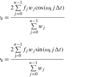
and phase associated with each frequencyωk=kω0 that is present in the Fourier decomposition of the function. They may be estimated from discrete data by
ak=
2
n−1
P
j=0
fjwjcos(ωkj 1t ) n−1
P
j=0
wj
(16)
bk=
2
n−1
P
j=0
fjwjsin(ωkj 1t ) n−1
P
j=0
wj
(17)
wherewj are the weights applied to each observation using
a window function. We used a Parzen window, which gives the weights as,
wj=1−
j−1 2(n−1) 1
2(n+1)
(18)
Press et al. (1992). In our analysis, we are interested in the diurnal frequency, with period,τ=24 h. For an analysis du-ration of 192 h, this corresponds to 8 cycles, or k=8. We estimated a8 andb8 from Eqs. (18) and (19). Noting the trigonometric identity
a8cos(8ω0t )+b8sin(8ω0t )=Asin(8ω0t+φ) (19) we can calculate
A=
q
a82+b28 (20)
and
φ= a8 |a8|
cos−1
b
8
A
(21) For negative values ofφ, we added 2π. The differences in the value ofφbetween the surface and each layer were used to calculate of the value ofz/dfor each layer from the sine term of Eq. (4). Similarly, the value ofz/dwas estimated from the natural log of the ratios of the amplitude at the layer’s temper-ature to the amplitude of the surface tempertemper-ature, considering the exponential decay term in Eq. (4). Knowing the vertical position of each measurement in the snowpack, we calcu-latedd, which provides a direct estimate of the diffusivity,k. Snowpack density (observed average of 260 kg m−3 in our study) and the specific heat of ice (2.09 kJ kg−1)were then used to estimate a value of conductivity,λ, from Eq. (2). The parameters estimated in this manner were used in the com-parisons between the equations used to estimate surface heat fluxes.
[image:5.595.50.197.507.637.2]21
-2000 -1500 -1000 -500 0 500
21-Jan 31-Jan 10-Feb 20-Feb 2-Mar 12-Mar 22-Mar 1-Apr
S
no
w
pac
k E
ner
gy
C
on
ten
t (
kJ
/m
2)
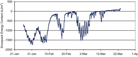
Figure 2. Snowpack energy content over time.
Fig. 2. Snowpack energy content over time.
For layers of the snowpack and soil between thermocouples, we used the average temperature between the thermocouples. Taking 0◦C ice as having 0 energy content, the energy con-tent without any liquid water present in the snowpack is,
U= hTsnowiWsnowρwCice+ hTsoiliρsoilCsoilDe (22)
wherehTsnowiis the depth averaged snow temperature and hTsoiliis the depth averaged soil temperature over the depth of the soil above the heat flux plate, De (0.1 m), Wsnow is the water equivalent of the snowpack (m), ρw is the
density of water (1000 kg m−3),ρsoil is the density of soil (1700 kg m−3),Ciceis the specific heat of ice (2.09 kJ kg−1) andCsoilis the specific heat of soil (2.09 kJ kg−1). This mea-sure of the energy content can only record energy content when there is no water in the snowpack; thus it can only reli-ably calculateU <0. For periods when U is greater than 0 due to the presence of liquid water in the snowpack, this Eq. (22) results in an underestimate that serves as a lower bound on
U. Figure 2 shows the snowpack energy content as measured by snowpack temperature over the study period; positive es-timates result from ground temperatures greater than 0 with a shallow snowpack.
Figure 3 shows the magnitude of heat fluxes at the sur-face of the snowpack inferred from the time series of energy content and measured ground heat flux necessary to explain the observed changes in snowpack energy content. During the first two weeks of the period, all parts of the snowpack were below freezing, so the energy content as measured by the temperature is an accurate description of the energy of the snowpack. During this period, there is an opportunity to examine how to model changes in snowpack energy that relate to the average snowpack temperature.
5 Results and discussion
5.1 Thermal properties
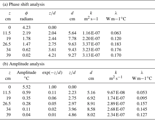
Table 1 presents thermal diffusivity values estimated from the Fourier analysis and an estimate of the conductivity based on the snowpack average density. The snow depth during this period was 39 cm and the analysis used the thermocouples at 0, 5, 12.5, 20, and 27.5 cm above the ground. The thermo-couple 35 cm above the ground was not used in the analysis
22
-150 -100 -50 0 50 100 150
26-Jan 5-Feb 15-Feb 25-Feb 7-Mar 17-Mar
S
no
w
S
ur
fa
ce
e
ner
gy
E
xc
han
ge (
kJ
/m
2/hr
)
(b
as
ed
o
n t
em
per
at
ur
e c
han
ge
s o
nl
y)
Figure 3. Snowpack surface energy fluxes over duration of study period reported at half-hourly intervals.
Fig. 3. Snowpack surface energy fluxes over duration of study
pe-riod reported at half-hourly intervals.
because the precision of its position relative to the snow sur-face was relatively worse and the results from it were unre-alistic, presumably due to this positioning inaccuracy. In Ta-ble 1a,zis the depth of the thermocouple from the snow sur-face;φis the phase of the temperature cycle from Eq. (21); andz/d is calculated based on the difference in phase be-tween the surface and the thermocouple using Eq. (4) Know-ingz, we have an estimate ofd, which is related to diffusiv-ity,k, byd=(2k/ω)1/2and finallyλby Eq. (2). In Table 1b the amplitude of the diurnal variation at each measurement point is calculated by Eq. (20), and the ratio of the amplitude at each layer to the amplitude at the surface gives exp(-z/d)
from Eq. (4). The log of this givesz/d, and the remainder of the calculations in Table 1b are the same as for Table 1a. The agreement (generally within 10%) between the results con-sidering just relative timing and those concon-sidering just rela-tive amplitude supports use of the Fourier analysis procedure with diurnal forcing.
As might be expected, the properties for the upper snow layers differ from those of the lower layers, suggesting an increase in effective conductivity that may be related to in-creases in density with depth. Although the heat Eq. (1) assumes homogeneity of snowpack thermal properties, it has been shown for heat conduction problems that a non-homogeneous diffusivity can be reasonably approximated by effective parameters in the heat equation within constraints of limited heterogeneity (Hanks et al., 1971).
[image:6.595.50.283.63.160.2] [image:6.595.310.545.64.175.2]Table 1. Effective thermal parameters averaged from surface to depth z using (a) timing and (b) amplitude information as independent
estimates. Conductivity was calculated using estimated density of 260 kg m−3.
(a) Phase shift analysis
z φ z/d d k λ
cm radians cm m2s−1 W m−1◦C
0 4.23 0.00
11.5 2.19 2.04 5.64 1.16 E-07 0.063
19 1.78 2.44 7.78 2.20 E-07 0.120
26.5 1.47 2.75 9.63 3.37 E-07 0.183
34 0.62 3.61 9.43 3.23 E-07 0.176
39 0.02 4.21 9.27 3.13 E-07 0.170
(b) Amplitude analysis
z Amplitude exp(−z/d) z/d d k λ
cm ◦C cm m2s−1 W m−1◦C
0 5.52 1.00 0.00
11.5 0.59 0.11 2.23 5.16 9.67 E-08 0.053
19 0.35 0.06 2.75 6.92 1.74 E-07 0.095
26.5 0.28 0.05 2.97 8.91 2.89 E-07 0.157
34 0.11 0.02 3.96 8.58 2.68 E-07 0.145
39 0.04 0.01 4.86 8.02 2.34 E-07 0.127
5.2 Model comparison
Equations (11–13) estimate the conductive heat flux at the surface of the snowpack as a function of the history of surface temperature and the current energy content of the snowpack. With direct measurements of the surface temperature and the ground heat flux, we were able to model the time evolution of snowpack energy content and surface heat conduction fluxes without examining the details of the surface energy balance (e.g. net radiation).
For Eq. (11), the equilibrium gradient equation, and Eq. (12), the force-restore equation, the independently esti-mated parameter value ofλ=0.058 W m−1◦C−1yielded very low energy contents relative to observations. However by changing the conductivity to 0.01 W m−1◦C−1for the equi-librium gradient (Eq. 11) and 0.007 W m−1◦C−1 for the force-restore (Eq. 12) approximate fits were possible (Fig. 4). These are unrealistically low thermal conductivity values, and result in severe damping of the daily variations in energy content. Equation (13), the modified force-restore equation, worked well with the conductivity independently estimated from the frequency analysis and calibratingωlf, with the re-sultant value corresponding to a period of 8.7 days, or using
dlf=(2k/ωlf)1/2, an effective depth of 16 cm. The suggestion is that physically realistic estimates of thermal conductivity from formulae (e.g. Sturm et al., 1997) could be used with such a model, leaving only a question about appropriate val-ues forωlf.
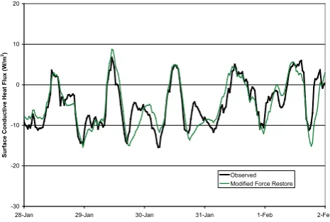
Comparing half-hourly surface heat flux estimates from the modified force-restore Eq. (13) to observations (Fig. 5) shows strong agreement to fluctuations at this time scale.
This comparison uses conductivity and half-hourly changes in internal energy (Fig. 3) derived from temperature measure-ments that include the surface temperature, so is not a com-pletely independent test of the model. Nevertheless, the mod-ified force restore result in Fig. 5 is derived primarily from the observed surface temperature and suggests the accuracy to which the conduction of energy into a snowpack can be parameterized in an energy balance snowmelt model based on surface temperature forcing alone. The largest disagree-ments are generally less than 10 W m−2in the early evening hours when the observed fluctuations in surface flux are not sinusoidal, but show an abrupt reduction in cooling. Records from a nearby airport suggest that this is likely related to the formation of fog at that time and the consequent reduction in net longwave losses (Luce, 2000).
Comparing surface heat flux estimates from all three equa-tions (Fig. 6) is more easily done with a 3-h average and shows that the equilibrium gradient approach (Eq. 11) pro-duces a damped and lagged signal relative to the observations and modified force-restore (Eq. 13), and the force-restore model (Eq. 12) is in phase but damped.
23
-2000 -1800 -1600 -1400 -1200 -1000 -800 -600 -400 -200
26-Jan 28-Jan 30-Jan 1-Feb 3-Feb 5-Feb 7-Feb 9-Feb
Ene
rgy
C
ont
ent
(k
J/
m
2)
Observed Equilibrium Gradient Force Restore Modified Force Restore
Figure 4. Measured and modeled energy content during first 2 weeks. Equilibrium gradient parameter used in Eq. 11 was λ = 0.01 W m-1oC-1. Force restore parameter used
in Eq. 12 was λ = 0.007 W m-1oC-1. Modified force restore parameters used in Eq. 13
were λlf = 0.058 W m-1oC-1, ωlf corresponding to 8.7 days, dlf=(2k/ωlf) = 16 cm.
Fig. 4. Measured and modeled energy content during first 2
weeks. Equilibrium gradient parameter used in Eq. 11 was
λ=0.01 W m−1◦C−1. Force restore parameter used in Eq. 12 was
λ=0.007 W m−1◦C−1. Modified force restore parameters used in
Eq. 13 wereλlf=0.058 W m−1◦C−1,ωlfcorresponding to 8.7 days,
dlf=(2k/ωlf)=16 cm.
24
-60 -50 -40 -30 -20 -10 0 10 20 30 40
28-Jan 29-Jan 30-Jan 31-Jan 1-Feb 2-Feb
Su
rf
ace C
on
du
ct
ive H
eat
F
lu
x (
W
/m
2)
Observed Modified Force Restore
Figure 5. Half-hourly surface conductive heat fluxes, observed and estimated from modified force-restore equation. Parameters used in Eq. 13 were λ = 0.058 W m-1oC-1,
ωlf corresponding to 8.7 days, dlf=(2k/ωlf) = 16 cm.
Fig. 5. Half-hourly surface conductive heat fluxes, observed and
estimated from modified force-restore equation. Parameters used in
Eq. 13 wereλ=0.058 W m−1◦C−1,ωlfcorresponding to 8.7 days,
dlf=(2k/ωlf)=16 cm.
conductivity, λ=0.025 W m−1◦C−1 and ωlf corresponding to a 3.7 day low frequency period, with effective depth
dlf=(2k/ωlf)1/2, of 7 cm. These adjustments push conduc-tivity just out of the range reported by Sturm et al. (1997). While calibration of both conductivity and low frequency period does improve the comparisons to measured energy fluxes, it is reassuring that using the directly measured con-ductivity and only calibratingωlf does result in quite good comparisons.
6 Conclusions
Heat flow through the snowpack is considered a difficult and complex process to model. So much so, that it has been generally assumed that single-layer snowpack models must,
25
-30 -20 -10 0 10 20
28-Jan 29-Jan 30-Jan 31-Jan 1-Feb 2-Feb
Su
rf
ace C
on
du
ct
ive H
eat
F
lu
x (
W
/m
2)
Observed Equilibrium Gradient Force Restore Modified Force Restore
Figure 6. Three-hour average surface conductive heat flux observations compared to three models over 5 day period. Equilibrium gradient parameter used in Eq. 11 was λ = 0.01 W m-1oC-1. Force restore parameter used in Eq. 12 was λ = 0.007 W m-1oC-1.
Modified force restore parameters used in Eq. 13 were λ= 0.058 W m-1oC-1, ω
lf
[image:8.595.50.282.60.222.2]corresponding to 8.7 days, dlf=(2k/ωlf) = 16 cm.
Fig. 6. Three-hour average surface conductive heat flux
observations compared to three models over 5 day
pe-riod. Equilibrium gradient parameter used in Eq. 11 was
λ=0.01 W m−1◦C−1. Force restore parameter used in Eq. 12 was
λ=0.007 W m−1◦C−1. Modified force restore parameters used in
Eq. 13 wereλ=0.058 W m−1◦C−1,ωlfcorresponding to 8.7 days,
dlf=(2k/ωlf)=16 cm.
26
-30 -20 -10 0 10 20
28-Jan 29-Jan 30-Jan 31-Jan 1-Feb 2-Feb
Su
rf
ace C
on
du
ct
ive H
eat
F
lu
x (
W
/m
2)
Observed Modified Force Restore
Figure 7. Three-hour average surface conductive heat flux observations compared to modified force restore formula calibrated to more closely approximate the diurnal range in surface heat fluxes. Parameters used in Eq. 13 were λ= 0.025 W m-1oC-1, ω
lf
corresponding to 3.7 days, dlf=(2k/ωlf) = 7 cm.
Fig. 7. Three-hour average surface conductive heat flux
observa-tions compared to modified force restore formula calibrated to more closely approximate the diurnal range in surface heat fluxes.
Param-eters used in Eq. 13 wereλ=0.025 W m−1◦C−1,ωlfcorresponding
to 3.7 days,dlf=(2k/ωlf)=7 cm.
[image:8.595.310.544.63.220.2] [image:8.595.50.283.307.463.2] [image:8.595.309.542.315.472.2]surface temperature in an energy balance snowmelt model. This formula calculates energy flux without detailed infor-mation on the distribution of temperature over depth, so presents a potential to approximate more complex multilayer models in applications where computational simplifications may be useful, as in lumped modeling of spatially heteroge-neous snowpacks. Our analysis shows a reasonable approx-imation in this case, and there would be benefit to testing against more complex models and observations in other en-vironments.
Following the logic of this approach to the extreme, we could recognize that the forcing at the surface could be de-composed into a Fourier series with multiple frequencies. Es-timation of the parameters for that series would use the time series of all previous surface temperatures – essentially the same information used in finite difference models. In prin-ciple the two numerical schemes would converge on a very similar answer. Within this concept lies the seed for simpli-fication. If we can recognize those few frequencies with the greatest power, we can continue to represent the snowpack as a single-layer, and only use such recent past temperature information as needed.
Acknowledgements. This work was supported by NASA Land
Surface Hydrology Program, grant number NAG 5-7597. The
views and conclusions expressed are those of the authors and should not be interpreted as necessarily representing official policies, either expressed or implied, of the US Government.
Edited by: W. Quinton
References
Anderson, E. A.: A Point Energy and Mass Balance Model of a Snow Cover, U.S. Department of Commerce, Silver Spring, Md.NOAA Technical Report NWS 19, 150 pp., 1976.
Arons, E. M. and Colbeck, S. C.: Geometry of heat and mass trans-fer in dry snow: a review of theory and experiment, Rev. Geo-phys., 33, 463–493, 1995.
Bartelt, P. and Lehning, M.: A physical SNOWPACK model for the Swiss avalanche warning Part I: numerical model, Cold Reg. Sci. Technol., 35, 123–145, 2002.
Berg, P. W. and McGregor, J. L.: Elementary Partial Differential Equations, Holden-Day, Oakland, 421 pp., 1966.
Bl¨oschl, G. and Kirnbauer, R.: Point Snowmelt Models with Differ-ent Degrees of Complexity – Internal Processes, J. Hydrol., 129, 127–147, 1991.
Colbeck, S. C.: An overview of seasonal snow metamorphism, Rev. Geophys. Space Ge., 20, 45–61, 1982.
Deardorff, J. W.: Efficient prediction of ground surface temperature and moisture with inclusion of a layer of vegetation, J. Geophys. Res., 83, 1889–1903, 1978.
Dickinson, R. E., Henderson-Sellers, A., and Kennedy, P. J.: Biosphere-Atmosphere Transfer Scheme (BATS) Version 1e as Coupled to the NCAR Community Climate Model, National Center for Atmospheric Research, Boulder, Colo.NCAR/TN-387+STR, 72 pp., 1993.
Gray, J. M. N. T., Morland, L. W., and Colbeck, S. C.: Effect of change in thermal properties on the propagation of a periodic thermal wave: application to a snow-buried rocky outcrop, J. Geophys. Res., 100, 15267–15279 , 1995.
Hanks, R. J., Austin, D. D., and Ondrechen, W. T.: Soil Temperature Estimation by a Numerical Method, Soil Sci. Soc. Am. Proc., 35, 665–667, 1971.
Horne, F. E. and Kavvas, M. L.: Physics of the spatially averaged snowmelt process, J. Hydrol., 191, 179–207, 1997.
Hu, Z. and Islam, S.: Prediction of Ground Surface Temperature and Soil Moisture Content by the Force-Restore method, Water Resour. Res., 31, 2531–2539, 1995.
Jin, J., Gao, X., Yang, Z.-L., Bales, R. C., Sorooshian, S., Dickin-son, R. E., Sun, S. F., and Wu, G. X.: Comparative Analyses of Physically Based Snowmelt Models for Climate Simulations, J. Climate, 12, 2643–2657, 1999.
Jordan, R.: A one-dimensional temperature model for a snow cover, Technical documentation for SNTHERM.89, US Army CRREL, Hanover, N.H. Special Technical Report 91–16, 49 pp., 1991. Koivasulo, H. and Heikinheimo, M.: Surface energy exchange over
a boreal snowpack: Comparison of two snow energy balance models, Hydrol. Process., 13, 2395–2408, 1999.
Luce, C. H., Tarboton, D. G., and Cooley, K. R.: Subgrid Parameter-ization Of Snow Distribution For An Energy And Mass Balance Snow Cover Model, Hydrol. Process., 13, 1921–1933, 1999. Luce, C.: Scale influences on the representation of snowpack
pro-cesses, Civil and Environmental Engineering, Utah State Univer-sity, Logan, Utah, 202 pp., 2000.
Luce, C. and Tarboton, D. G.: The Application of Depletion Curves for Parameterization of Subgrid Variability of Snow, Hydrol. Pro-cess., 18, 1409–1422, 2004.
Marks, D., Domingo, J., Susong, D., Link, T., and Garen, D.: A spa-tially distributed energy-balance snowmelt model for application in mountain basins, Hydrol. Process., 13, 1935–1959, 1999. Nash, J. E. and Sutcliffe, J. V.: River Flow Forecasting Through
Conceptual Models, 1. A Discussion of Principles, J. Hydrol., 10, 282–290, 1970.
Press, W. H., Teukolsky, S. A., Vetterling, W. T., and Flannery, B. P.: Numerical Recipes in FORTRAN: The Art of Scientific Comput-ing, Second Edn., Cambridge University Press, New York, 1992. Sturm, M., Holmgren, J., K¨onig, M., and Morris, K.: The thermal
conductivity of seasonal snow, J. Glaciol., 43, 26–41, 1997. Tarboton, D. G.: Measurement and Modeling of Snow Energy
Bal-ance and Sublimation From Snow, International Snow Science Workshop Proceedings, Snowbird, Utah, 260–279, 1994. Tarboton, D. G., Chowdhury, T. G., and Jackson, T. H.: A Spatially
Distributed Energy Balance Snowmelt Model, Biogeochemistry of Seasonally Snow-Covered Catchments, Boulder, Colo., 141– 155, 1995.
Tarboton, D. G. and Luce, C. H.: Utah Energy Balance Snow Ac-cumulation and Melt Model (UEB), Computer model techni-cal description and users guide, Utah Water Research Labora-tory and USDA Forest Service Intermountain Research Station, http://www.engineering.usu.edu/dtarb/, last access: 17 August 2009, 1996.