An artificial neural network model for rainfall forecasting in Bangkok, Thailand

www.hydrol-earth-syst-sci.net/13/1413/2009/ © Author(s) 2009. This work is distributed under the Creative Commons Attribution 3.0 License.

Earth System

Sciences

An artificial neural network model for rainfall forecasting in

Bangkok, Thailand

N. Q. Hung, M. S. Babel, S. Weesakul, and N. K. Tripathi

School of Engineering and Technology, Asian Institute of Technology, Thailand

Received: 14 December 2007 – Published in Hydrol. Earth Syst. Sci. Discuss.: 30 January 2008 Revised: 29 June 2009 – Accepted: 27 July 2009 – Published: 7 August 2009

Abstract. This paper presents a new approach using an Arti-ficial Neural Network technique to improve rainfall forecast performance. A real world case study was set up in Bangkok; 4 years of hourly data from 75 rain gauge stations in the area were used to develop the ANN model. The developed ANN model is being applied for real time rainfall forecast-ing and flood management in Bangkok, Thailand. Aimed at providing forecasts in a near real time schedule, different network types were tested with different kinds of input in-formation. Preliminary tests showed that a generalized feed-forward ANN model using hyperbolic tangent transfer func-tion achieved the best generalizafunc-tion of rainfall. Especially, the use of a combination of meteorological parameters (rela-tive humidity, air pressure, wet bulb temperature and cloudi-ness), the rainfall at the point of forecasting and rainfall at the surrounding stations, as an input data, advanced ANN model to apply with continuous data containing rainy and non-rainy period, allowed model to issue forecast at any mo-ment. Additionally, forecasts by ANN model were compared to the convenient approach namely simple persistent method. Results show that ANN forecasts have superiority over the ones obtained by the persistent model. Rainfall forecasts for Bangkok from 1 to 3 h ahead were highly satisfactory. Sen-sitivity analysis indicated that the most important input pa-rameter besides rainfall itself is the wet bulb temperature in forecasting rainfall.

1 Introduction

Accurate information on rainfall is essential for the planning and management of water resources. Additionally, in the ur-ban areas, rainfall has a strong influence on traffic, sewer

Correspondence to: N. Q. Hung

(nguyenquang.hung@ait.ac.th)

systems, and other human activities. Nevertheless, rainfall is one of the most complex and difficult elements of the hydrol-ogy cycle to understand and to model due to the complexity of the atmospheric processes that generate rainfall and the tremendous range of variation over a wide range of scales both in space and time (French et al., 1992). Thus, accurate rainfall forecasting is one of the greatest challenges in opera-tional hydrology, despite many advances in weather forecast-ing in recent decades (Gwangseob and Ana, 2001).

Toth et al. (2000) compared short-time rainfall prediction models for real-time flood forecasting. Different structures of auto-regressive moving average (ARMA) models, artifi-cial neural networks and nearest-neighbors approaches were applied for forecasting storm rainfall occurring in the Sieve River basin, Italy, in the period 1992-1996 with lead times varying from 1 to 6 h. The ANN adaptive calibration appli-cation proved to be stable for lead times longer than 3 hours, but inadequate for reproducing low rainfall events.

Koizumi (1999) employed an ANN model using radar, satellite and weather-station data together with numerical products generated by the Japan Meteorological Agency (JMA) Asian Spectral Model and the model was trained us-ing 1-year data. It was found that the ANN skills were better than the persistence forecast (after 3 h), the linear regression forecasts, and the numerical model precipitation prediction. As the ANN model was trained with only 1 year data, the re-sults were limited. The author believed that the performance of the neural network would be improved when more train-ing data became available. It is still unclear to what extent each predictor contributed to the forecast and to what extent recent observations might improve the forecast.

Past studies have obviously indicated that ANN is a good approach and has a high potential to forecast rainfall. The ANN is capable to model without prescribing hydrological processes, catching the complex nonlinear relation of input and output, and solving without the use of differential equa-tions (Luk et al., 2000; Hsu et al., 1995; French et al., 1992). In addition, ANN could learn and generalize from examples to produce a meaningful solution even when the input data contain errors or is incomplete (Luk et al., 2000). Most of the existing ANN models applied in rainfall forecasting are event based; the models were fed in input with screened/generated data that contained only rainy periods (i.e., rainfall events, rainy days or monthly rainfall data). By using only the data from the rainy periods as training data, ANN models could easily identify the patterns characterizing the rainfall. How-ever, on the other hand, any features or characteristics not in-cluded within the training data will not be learned by ANN. Translated this means that conventional ANN models could only issue accurate forecasting when rain occurred already and they can estimate how long the rain would last, but they are unable to predict whether it would rain or not if there is no rain at the time of issuing forecast. Hence, most of the previ-ous studies of ANN on rainfall forecast are not fully suitable for the application in real time forecasting.

The main objective of this study is to develop a rainfall forecast model using ANN technique. The developed ANN model is designed to run a real time task, in this situation, the input to the model should not be event based data but con-secutive data including non-rainy periods to acquire a fully representation of both rain and no rain conditions. When us-ing only continuous past rainfall data to train an ANN model, no rain periods with zero values make no change in weights update process so the ANN could not recognize the pattern

and provided poor forecasting results. Targeting to explore alternative ways to overcome this problem, several models were tested by changing model architecture, transfer function and employing additional data as input variables. Results of preliminary test showed that with the use of additional data (meteorology data and rainfall record from surrounding sta-tions), a continuous ANN model could perform highly accu-racy of rainfall forecast and can be used for real time appli-cations. Applying the developed ANN model, rainfall from 1 to 6 h ahead was forecasted at 75 rain gauge stations (as fore-cast point) in Bangkok city, Thailand, using present hourly rainfall data and meteorological parameters of relative hu-midity, air pressure, wet bulb temperature, cloudiness, and rainfall from surrounding rain gauge stations as input vari-ables. Additionally, along with the ANN model, a persistent model was developed and compared with the predictions of the ANN model in order to reveal the real advantage of the continuous ANN model in term of real time forecast. Sensi-tivity analysis is also carried out to identify the most and least important factors in predicting rainfall in the study area.

2 Study area

Bangkok, the capital and commercial city of Thailand, is one of the highly developed cities in Southeast Asia. Having a land area of 1569 km2, it is located in the central part of the Thailand on the floodplain of the Chao Phraya River, with latitude 13.45 N and longitude 100.35 E. The area has a trop-ical type of climate with long hours of sunshine, high tem-peratures and high humidity. There are three main seasons; rainy (April-October), winter (November–January) and sum-mer (February–March). The average minimum temperature is approximately in low to mid 20 s◦C and high temperature in mid 30s◦C. Bangkok receives an average annual rainfall of 1500 mm and is influenced by the seasonal monsoon. The city is affected by the flood on regular basis due to rainfall, which paralyzes most of the daily activities. Some of the immediate consequences of a heavy rainfall in Bangkok are: water clogging in the streets, heavy traffic jams, blackouts, and direct or indirect economic losses.

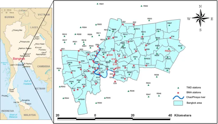
Fig. 1. Location of the study area and the rain gauge stations network.

information and the failure of gravity to effectively remove drainage water from the city make urban flooding inevitable during the wet season. For the city like Bangkok, one of the best ways to cope with the flooding problem is to provide ad-vance rainfall forecasting and flood warning. Knowing the condition of rainfall in Bangkok in advance can help in man-aging and dealing with problems due to flooding.

The Department of Drainage and Sewage (DDS) of the Bangkok Metropolitan Administration (BMA) had estab-lished the Bangkok Metropolitan Flood Control Center (FCC) in 1990 for systematic and efficient management of operation and control of flood protection facilities. The BMA has 53 online rain gauge stations scattered through-out Bangkok and sensors installed at canal gates and pump-ing stations that observe water level. The observed data is transferred in real time to the FCC by ultra high frequency radio signals every 15 min. Besides, the Thai Meteorological Department (TMD) owns a network of 51 rain gauge sta-tions covering Bangkok and nearby areas. Both rain gauge networks consist of rain gauges of tipping bucket type with 0.5 mm accuracy. Furthermore, Bangkok has one 100-m tall meteorological mast station covered the area. Data collected at the meteorological station was transmitted via a dedicated telephone line to a central processing computer for data stor-age and analysis. These data are now available on the Internet and can be used for online applications. Locations of the rain gauges are shown in Fig. 1.

There was actually no reliable rainfall forecast mechanism using rain gauge data in the past. Based upon the histori-cal data and the current situation, the flood forecast analysis is manually carried out at the FFC. After a decision about control policy is made out of this analysis, the flood con-trol protection command is then broadcasted to all remote

control stations (gates and pumping stations). This system is acceptable in terms of real time data transmission but not efficient in terms of urban flood forecast and flood manage-ment. Therefore, there is a need to investigate and apply an accurate technique for real time rainfall forecasting. ANN with its advantages such as computation speed, learning ca-pability, fault tolerance and adoptability, has been selected to be a tool for short-term rainfall forecast using rain gauge data for Bangkok area. The model is mimic design, so it can be applied not only to Bangkok area but also to other tropical developing urban areas as well.

Historical rainfall data was collected from 104 stations of the BMA and TMD rain gauge networks for the period from 1991 to 2005. After analyzed data, the period from 1 Jan-uary 1997 to 31 December 1999 was selected to train ANN models, and the data of the year 2003 were used as a test-ing set. This study focus on the Bangkok area only, so to-tal 75 stations inside Bangkok area were selected, while the other 29 stations which are located outside Bangkok were discarded, it roughly made each selected station representing for an area around 21 km2. The collected meteorological data which contained hourly measurements of six parameters ob-served in the mast station, that is: relative humidity, wet bulb temperature, dry bulb temperature, air pressure, cloudiness, and wind speed for the same period as rainfall data. As an additional variable, the average hourly rainfall intensity of all the rain gauges was simply arithmetically average computed and provided with the meteorology data.

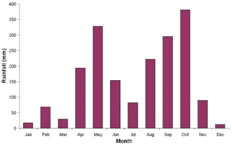
Fig. 2. Average monthly rainfall in Bangkok.

the average maximum RH of 93% and the average minimum RH of 52%. The average annual temperature is 26.8◦_{C, with} the average maximum temperature of 33.4◦_{C in April and} the average minimum temperature of 20.4◦C in December. The average annual rainfall is 1869.5 mm with the highest average monthly rainfall of approximately 381 mm observed in October, and the lowest average monthly rainfall of about 12 mm occurring in December, usually the driest month of the year.

3 Artificial neural network

An artificial neural network (ANN) is an interconnected group of artificial neurons that has a natural property for stor-ing experiential knowledge and makstor-ing it available for use. The first simplest form of feedforward neural network, called perceptron has been introduced by Rosenblatt in 1957. This original perceptron model contained only one layer, inputs are fed directly to the output unit via the weighted connec-tions. Although the perceptron initially seemed promising, it was eventually proved that perceptrons could not be trained to recognize many classes of patterns. After that, multilayer perceptron (MLP) model was derived in 1960 and gradually became one of the most widely implemented neural network topologies. Multilayer perceptron means a feedforward net-work with one or more layers of nodes between the input and output nodes. The MLP overcomes many limitations of the single layer perceptron, their capabilities stem from the non-linear relationships among the nodes (Lippmann, 1987). In theirs study of nonlinear dynamics, Lapedes and Farber (1987) have pointed out the important that the MLP is ca-pable of approximating arbitrary functions. Two important characteristics of the MLP are: its nonlinear processing ele-ments (PEs) which have a nonlinearity that must be smooth (the logistic function and the hyperbolic tangent are the most widely used); and their massive interconnectivity (i.e. any element of a given layer feeds all the elements of the next layer).

Fig. 3. A simple generalized feedforward neural network with

hy-perbolic tangent function.

Generalized feedforward networks are a generalization of the MLP such that connections can jump over one or more layers. In theory, a MLP can solve any problem that a gen-eralized feedforward network can solve. In practice, how-ever, generalized feedforward networks often solve the prob-lem much more efficiently. A classic example of this is the two-spiral problem. Without describing the problem, it suf-fices to say that a standard MLP requires hundreds of times more training epochs than the generalized feedforward net-work containing the same number of processing elements. A simple generalized feedforward neural network with two hidden layers is shown in Fig. 3.

input node, andmis the number of output node. The num-ber of input and output nodes is problem-dependent, and the number of input nodes depends on data availability. In addi-tion, the selection of input should be based on priori knowl-edge of the problem. A firm understanding of the hydrologic system under consideration is necessary for the effective se-lection of input data (Ahmad and Simonovic, 2005).

Regarding the second issue, several training processes are available to find the values of connection weights. These al-gorithms differ in how the weights are obtained. The selec-tion of training algorithm is related to the network type, com-puter memory, and the input data. There are several training algorithms which can be randomly listed as follow: Quick-Prop (QP), Orthogonal Least Square (OLS), Levemberg-Marquart (LM), Back Propagation (BP), and Resilient Prop-agation Algorithm (RPROP). As implied in this study, the standard back propagation algorithm is used in ANN train-ing based on its most popular success, Coulibaly et al. (2000) stated that 90% of ANN models applied in the field of hydrol-ogy used the back propagation algorithm. In fact the renewed interest in ANN was in part triggered by the existence of back propagation which was first introduced by Werbos in 1974 for the three layer perceptron network. The application area of the MLP network remained rather limited until the break-through in 1986 when Rumelhart and McClelland published theirs work with back propagation and gained recognition. The back propagation rule propagates the errors through the network and allows adaptation of the hidden units. This al-gorithm involves minimizing the global error by using the steepest descent or gradient approach. The network weights and biases are adjusted by incrementing the negative gradient of the error function for each iteration.

The multilayer perceptron is trained with error-correction learning, which means that the desired response for the sys-tem must be known. The error correction learning works in the following way: from the system responsedi(n)at nodei

at iterationn,and the desired responseyi(n)for a given input

pattern, an instantaneous errorei(n)is defined by

ei(n)=di(n)−yi(n) (1)

Using the theory of gradient-descent learning, each weight in the network can be adapted by correcting the present value of the weight with a term that is proportional to the present input and error at the weight, i.e. the weight from nodej to nodei(wij) can be calculated by:

wij(n+1)=wij(n)+ηδi(n)xj(n) (2)

where,xjis a transform function at nodej,iandj indicate

different layers.

The local errorδi(n)can be directly computed fromei(n)

at the output node or can be computed as a weighted sum of errors at the internal nodes. The constantηis called the step size. Most gradient search procedures require the selection of step size. The larger step size, the faster the minimum can

be reached. However, if the step size is too large, then the algorithm will diverge and the error will increase instead of decrease. If the step size is too small then it will take too long to reach the minimum, which also increases the probability of getting caught in local minima. Momentum learning is an improvement to the straight gradient descent in the sense that a memory term (the past increment to the weight) is used to speed up and stabilize convergence. In momentum learning the equation to update the weights becomes

wij(n+1)=wij(n)+ηδi(n)xj(n)+α(wij(n)−wij(n−1))(3)

whereα is the momentum. Normallyα should be set be-tween 0.1 and 0.9. The back propagation algorithm is applied as follow:

1. Initialize all weights and bias (normally a small random value) and normalize the training data.

2. Compute the output of neurons in the hidden layer and in the output layer (net) using

neti =

X

wijxi +θi ; θi is a bias forP Ei (4)

1. Compute the error and weight update.

2. Update all weights, bias and repeat steps 2 and 3 for all training data.

3. Repeat steps 2 to 4 until the error converges to an ac-ceptable level.

4 ANN models in preliminary test

Table 1. Alternative ANN models considered in the study.

Model Network type Transfer function Architecture Training data

A Simple multilayer perceptron Sigmoid 5-5-5-1 Rt−4, Rt−3, Rt−2, Rt−1, and Rt

B Simple multilayer perceptron Sigmoid 5-10-10-1 Rt−4, Rt−3, Rt−2, Rt−1, and Rt

C Generalized feedforward Sigmoid 5-10-10-1 R_t−4, Rt−3, Rt−2, Rt−1, and Rt

D Generalized feedforward Sigmoid 6-16-12-1 Rt, RHt, WBTt, APt, CLt, and ARt

E Generalized feedforward Hyperbolic Tangent 6-18-12-1 Rt, RHt, WBTt, APt, CLt, and ARt

F Generalized feedforward Hyperbolic Tangent 9-22-11-1 Rt, RHt, WBTt, APt, CLt, ARt, SR1t, SR2t, and SR3t

G Generalized feedforward Hyperbolic Tangent 9-22-11-1 Same as Model F but only rainfall events

Rt= Rainfall intensity att, RHt= Relative humidity att, WBTt= wet bulb temperature att, APt= Air pressure att, CLt= Cloudiness att,

ARt= Average hourly rainfall intensity of all rain gauges att, and SR1t= Rainfall intensity at surrounding station 1 att.

training set was used to calibrate the weights of the network; the cross validation set was used to monitor the progress of training process. The testing data set which used for the final evaluation of the model performance is the hourly rainfall records of the year 2003. Presented in this section are six distinctive alternative models, whose structure and result are considered as the most presentable for the preliminary test, details of these six ANN models are summarized in Table 1. The first model (Model A) used the multilayer perceptron (MLP) network with a simple structure involving five nodes in the input layer, two hidden layers having 5 hidden nodes in each of the two layers, and one node in the output layer (5-5-5-1). Inputs to the model were hourly rainfall data (at time t) and past hourly rainfall with four hourly lag times i.e., from (t−4) to (t-1) at station E18, while the output is the rainfall intensity of the next hour (t+1). The transfer function in nodes was the sigmoid function. For the second model (Model B), the network type, transfer function and input data were kept as same as Model A but the number of hidden nodes in both hidden layers was increased from 5 to 10.

In the third model (Model C), the generalized feedforward network was employed, the input variables, transfer function and network architecture (5-10-10-1) were similar as Model B. The fourth model (Model D) also adopted the generalized feedforward network, with the sigmoid transfer function, but different input variables and model structure. Theoretically, the self-learning nature of ANN normally allows it to pre-dict without extensive prior knowledge of all processes in-volved. However, a good understanding of the physical pro-cesses involved, and a hypothesis on how different propro-cesses (and their state variable) interact with each other would help in identifying parameters used in the input data. Thus, other meteorological parameters were added to the input data set and the past rainfall data was excluded as it brings more zero values to the training process (no rain periods). This resulted in six input variables for Model D, which included present time values of relative humidity, wet bulb temperature, air pressure, cloudiness, average hourly rainfall intensity of all the rain gauge stations, and present rainfall at the station E18. The model structure was modified to 6 input nodes, 16 and

12 hidden nodes in the first and second hidden layer, respec-tively, and 1 output node (6-16-12-1).

In the fifth model (Model E), the input data was remained as same as in Model D but the hyperbolic tangent function was used instead of the sigmoid function and the number of hidden node in the first layer was increased to 18, which formed a new network architecture (6-18-12-1). In the sixth model (Model F), spatial data were also considered in the in-put variables for the ANN model, rainfall data of stations around E18 were included to the input that were used in Model D and E. A correlation analysis was carried out for 75 selected rain gauge stations to determine which stations are strongly related to the station E18. Results of the analy-sis revealed higher correlation of the stations E00, E19 and E26 with the station E18. Therefore, the present hourly rain-fall data of these three stations were added to the input data set of Model E in the formulation of Model F. The change in the input variables resulted in an increase in the number of nodes in the input layer to 9, increase in the number of nodes to 22 in the first hidden layer and 11 in the second hidden layer.

5 Results and discussion

5.1 Comparison of models for one-hour ahead rainfall forecast at station E18

The one-hour ahead forecast accuracy of the six ANN mod-els in preliminary testing stage (model A to F) were evalu-ated using to Efficiency Index (EI), Root Mean Square Error (RMSE), and Correlation Coefficient (R2); the behavior of these parameters is presented in Table 2. To investigate the models deeper in terms of quantitative forecast, all the pat-terns with no rain in observed data were excluded, and model performance indices based on the remaining data (rainy pe-riods only) were re-evaluated and the results are shown in Table 3.

Fig. 4. Scatter plot of observed and forecasted rainfall for Model A and Model B (testing stage).

Fig. 5. Scatter plot of observed and forecasted rainfall for Model C and Model D (testing stage).

Table 2. Performance statistics of the six ANN models for 1 h

rain-fall forecasting at E18 station.

Model A B C D E F

Index Training (1997, 1998 and 1999 data) EI (%) 31.62 40.46 50.5 62.47 81.52 98.54 RMSE (mm/h) 2.15 1.96 1.75 1.51 0.98 0.53 R2 0.48 0.54 0.57 0.68 0.87 0.98

Testing (2003 data)

EI (%) 28.35 38.25 48.32 59.19 80.54 96.72 RMSE (mm/h) 2.1 1.98 1.86 1.56 1.05 0.71 R2 0.41 0.49 0.55 0.66 0.83 0.94

models. This was attributed to the fact that the cross vali-dation approach was helpful in detecting the best general-ization point. The first three ANN models (A, B, C), which used only the characteristics of previous rainfall value as in-put variables, provided very low accuracy of forecast. The lowest score was obtained by Model A since the number of hidden nodes was insufficient to memorize and learn the

pat-tern of training data. Although the number of hidden nodes was increased from 5 to 10 in each hidden layer in Model B, improvement in the result was minor. Changing the net-work type in Model C enhanced the performance compared to Model A and B. This suggests that the generalized feed-forward network performed better than the simple multilayer perceptron network in this study. Figures 4 and 5 depict the scatter plot of rainfall forecast against the observed record of these three models, showing that most low rainfalls are over-estimated and high rainfalls are underover-estimated. These three models rendered several errors in forecasts; sometimes they provided rainfall forecasts when there was no rain. No rain in forecasted results versus no rain in the observed record was considered as a very high forecasting result; therefore, when the non-rainy period was excluded for quantitative investi-gation, the EI and coefficient of correlation were degraded as presented in Table 3. All these results of the first three models A, B and C (Tables 2 and 3) indicated that rainfall-rainfall model structure is not working well in the approach of a continuous model.

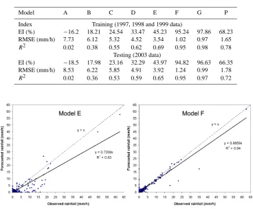
Table 3. Performance statistics of models for 1h rainfall forecasting at E18 station (rainfall events only).

Model A B C D E F G P

Index Training (1997, 1998 and 1999 data)

EI (%) −16.2 18.21 24.54 33.47 45.23 95.24 97.86 68.23

RMSE (mm/h) 7.73 6.12 5.32 4.52 3.54 1.02 0.97 1.65

R2 0.02 0.38 0.55 0.62 0.69 0.95 0.98 0.78

Testing (2003 data)

EI (%) −18.5 17.98 23.16 32.29 43.97 94.82 96.63 66.35

RMSE (mm/h) 8.53 6.22 5.85 4.91 3.92 1.24 0.99 1.78

R2 0.02 0.36 0.53 0.59 0.65 0.95 0.97 0.72

Fig. 6. Scatter plot of observed and forecasted rainfall for Model E and Model F (testing stage).

different input variables, brought a very interesting outcome. The combination of the meteorology information with rain-fall series in the input data has generally improved model per-formance as the Model D yielded better results than Model C for both the training and testing phase. For model E, re-markable performance indicates that with hyperbolic tangent function, model E is capable of generalizing better results from the same set of input variables than model D, which use the sigmoid function. Models D and E also show degraded performance indices, just as models A, B and C, when no-rain data was eliminated (Table 3). Figs. 5 and 6 reveal that both models E and D provided underestimated rainfall fore-casts.

Model F, which involved the input data of rainfall at the station of forecast and the three surrounding stations, as well as other meteorological parameters (Table 1), produced the highest performance (Table 2). The scatter plot in Figure 6 confirms the match between forecasted and observed rainfall. Moreover, Model F also worked well when applied to each rainfall event (Table 3). The high accuracy result by Model F (Tables 2 and 3) again highlights the importance of using additional data to enable the ANN model to train and run in continuous mode.

In order to evaluate the superiority of the optimal model (Model F) over the conventional approach in the real time rainfall forecast, two other models were developed. The first model is Model G with the same setup as Model F, but using only rainfall events to feed in input as given in Table 1. The second model is a persistence approach (Model P), or na¨ıve prediction, widely used in forecasting theory. This predictive scheme, which simply substitutes the last measured values as the current forecast, represents a good bottom line bench-mark.

Fig. 7. Scatter plot of observed and forecasted rainfall for Model G (testing stage).

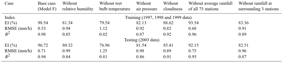
Table 4. Performance statistics for sensitivity analysis for 1 h rainfall forecasting at E18 station.

Case Base case Without Without wet Without Without Without average rainfall Without rainfall at (Model F) relative humidity bulb temperature air pressure cloudiness of all 75 stations surrounding 3 stations

Index Training (1997, 1998 and 1999 data)

EI (%) 98.54 81.34 79.54 82.13 88.62 93.54 83.36

RMSE (mm/h) 0.53 0.94 1.12 0.92 0.82 0.68 0.91

R2 0.98 0.85 0.82 0.87 0.92 0.96 0.89 Testing (2003 data)

EI (%) 96.72 80.32 76.96 81.54 85.41 92.15 82.51

RMSE (mm/h) 0.71 0.99 1.25 0.98 0.89 0.75 0.96

R2 0.94 0.84 0.81 0.86 0.91 0.95 0.87

Examination of Table 3 also reveals that the performance of the persistent model (Model P) gained the third place among eight presented models. However, since the persis-tent model considered the forecast equal to the last rainfall record, it always issued lag forecast and the performance in-dices of Model P were significantly less than that of Model F (Table 3). As a feature of a tropical climate, rainfall in Bangkok is rapid, with high fluctuation in both duration and intensity; therefore, the persistent approach is inadequate to provide applicable forecasts for real time purposes.

Comparison of Model G and persistent model with Model F confirmed that when applied for rainy data only, Model F had comparable performance with Model G and was much better than Model P. In the case of using continuous data, model F has outperformed both Model G and P.

5.2 Sensitivity analysis

While training a network, the effect that each of the network inputs has on the network output should be studied. This provides feedback as to which input parameters are the most significant. Based on this feedback, it may be decided to prune the input space by removing the insignificant parame-ters. This also reduces the size of the network, which in turn reduces the network complexity and the training time. The

sensitivity analysis is carried out by removing each of the input parameters in turn from the input parameters used on Model F and then comparing the performance statistics, EI, RMSE andR2. The greater the effect observed in the output, the greater is the sensitivity of that particular input parameter. As mentioned earlier, the inputs into Model F included rainfall (mm/h) at the station E18, relative humidity (%), wet bulb temperature (◦C), air pressure (HPa), total cloudiness, arithmetical average rainfall (mm/h) of all rain gauges, and rainfall (mm/h) from the three surrounding stations (strongly connected with station E18). The rainfall on the particular station was considered as the main parameter; hence this pa-rameter was not included in the sensitivity analysis. The top three strongly connected stations (E00, E19 and E26) to E18 station were selected based on the correlation and were con-sidered to have the same relative importance level as the cor-relation coefficients are 0.91, 0.93 and 0.87, respectively. For this reason, in the sensitivity analysis, these three stations were excluded once, which formed an ANN structure (6-18-12-1). For the remaining five cases, the same network ar-chitecture (8-22-11-1), using the hyperbolic tangent function and forecasting rainfall 1 hour ahead is used (Table 4).

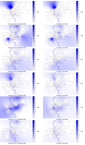
Fig. 8. Comparison of observed rainfall (left side maps) and predicted rainfall (right side maps) for 1 to 6 h ahead forecasting on 16 September

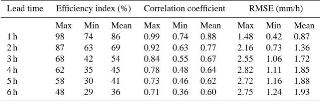
Table 5. Summary of ANN results for rainfall forecasting at 75 rainfall stations (Model F).

Lead time Efficiency index (%) Correlation coefficient RMSE (mm/h)

Max Min Mean Max Min Mean Max Min Mean

1 h 98 74 86 0.99 0.74 0.88 1.48 0.42 0.87

2 h 87 63 69 0.92 0.63 0.77 2.16 0.73 1.36

3 h 68 42 54 0.84 0.55 0.67 2.55 1.06 1.72

4 h 62 35 45 0.78 0.48 0.64 2.82 1.11 1.85

5 h 58 30 41 0.73 0.46 0.62 2.72 1.16 1.88

6 h 48 29 36 0.71 0.36 0.60 2.75 1.24 1.93

wet bulb temperature gave similar results: EI received the lowest value. This indicates that the most significant input is wet bulb temperature. Likewise, from overall performance of models in Table 4, the second most important parameter is the relative humidity, while other important parameters are the air pressure and the rainfall at the three surrounding sta-tions. The cloudiness remained as the fifth most important parameter, with an EI decreasing to 88.62% for the model without this parameter. The ANN model without average rainfall of all stations gave EI of 93.54% in the training stage, nearest to the results of Model F, indicating that this input data contributed the least in improving the model results. 5.3 Rainfall forecasting from 1 to 6 h for Bangkok area

From the preliminary test, Model F was identified as the best model among six ANN testing models. The efficiency at-tained at 1 h ahead forecast is highly accurate; the scatter plot in Fig. 6 also shows that peaks forecast are matched with observed data. Therefore, Model F was selected to forecast rainfall at lead times of one to six hours at all 75 rain gauge stations in Bangkok. The same training approach and data selection of the preliminary test was implemented in the fore-casting stage.

Table 5 presents the summarized ANN model results in terms of maximum, minimum, mean EI,R2, and RMSE for rainfall forecasting from 1 to 6 h ahead at all 75 rain gauge stations. The models performed consistently well, providing stable and similar results for all stations. It is seen that the model performance decreases with the increasing lead time of the forecast. This is to be foreseen, as the ANN model uses a recursive method to forecast multi-step ahead. Thus the forecast errors are propagated and accumulated from step to step.

It can further be seen that the ANN models provide re-markably acceptable results of rainfall forecasts for 1 and 2 h ahead (Table 5). For 1 h lead forecasts at some stations the value of EI reached up to 98%, while the lowest EI value of all stations was 74%. Similarly, the maximum and minimum correlation coefficient values of 0.99 and 0.74 reflect highly satisfactory results. For 2 h ahead forecast, the results may

also be considered quite satisfactory with maximum EI of 87%, and minimum EI of 63%; and maximum and minimum

R2of 0.92 and 0.63 respectively. Forecasting results of 3 h ahead are less satisfactory, results for 4 to 6 h ahead may be considered to be poor with the mean EI varying between 45 and 36% and meanR2in the range from 0.78 to 0.71.

Observed rainfall (left figures) and the predicted rainfall (right figures) for 1 to 6 h ahead forecasting on the rainfall event on 16 September 2003 are compared in Fig. 8. These maps are developed with the known geographical locations and the observed and forecasted rainfall at all 75 stations for clear visualization and comparison. The Kriging method was employed for interpolation of the scattered data over the study area.

6 Conclusions

In this study, an Artificial Neural Network model was em-ployed to forecast rainfall for Bangkok, Thailand, with lead times of 1 to 6 h. Comparison of 1 h ahead rainfall forecast of the six models considered in the preliminary test showed that a combination of meteorological parameters such as relative humidity, air pressure, wet bulb temperature, and cloudiness, along with rainfall data at the forecasting station and other surrounding stations, as an input for the model could signifi-cantly improve the forecast accuracy and efficiency. Results of preliminary tests also concluded that the generalized feed-forward network and hyperbolic tangent function performed well in this study. With the appropriate network architec-ture and especially with the use of auxiliary data, the ANN model was able to learn from continuous input data which contained both rain and dry periods, thus the model can be adopted to run for real time forecasting. The superiority in performance of the ANN model over that of the persistent model again confirmed that the real advantage of a continu-ous ANN model is that it can provide a satisfactory rainfall forecast at any moment.

It is important to determine the dominant model inputs, as this increases the generalization of the network for a given data. Furthermore, it can help reduce the size of the network and consequently reduce the training time. In this study, sen-sitivity analysis was used to rank the input parameters with respect to their importance in forecasting rainfall based on the model performance. Results of the sensitivity analysis indicated that the most important input parameter, besides rainfall itself, is the wet bulb temperature; further study over the entire rain gauge network could be carried out for more significant conclusions.

The ANN model was found to be efficient in fast compu-tation and capable of handling the noisy and unstable data that are typical in the case of weather data. The predicted values of all 75 rain gauge stations matched well with the observed rainfall for forecasts with short lead times of 1 or 2 h. Not only that, the rainfall forecasting for 3 h ahead using the ANN model also provided reasonably acceptable results. The efficiency indices were gradually reduced as the forecast lead time increased from 4 to 6 h. Although the model perfor-mance of 6 hour forecasting was low and the forecasting was not as accurate as expected, the developed model can still be used for practical applications such as rainfall forecasting and flood management for the urban areas.

Acknowledgements. This article is a part of doctoral research con-ducted by the first author at Water Engineering and Management, Asian Institute of Technology, Bangkok, Thailand. The financial support provided by the DANIDA for pursuing the study is gratefully acknowledged. The author would like to express sincere gratitude to the staff of the Thai Meteorological Department and the Bangkok Metropolitan Administration for providing, sourcing and facilitating access to and usage of invaluable data and information used in this study. Thanks are also extended to the anonymous

reviewer and the editor for their constructive contributions to the manuscript.

Edited by: E. Toth

References

Abrahart, R. J. and See, L.: Comparing neural network and autore-gressive moving average techniques for the provision of contin-uous river flow forecast in two contrasting catchments, Hydrol. Proc., 14, 2157–2172, 2000.

Ahmad, S. and Simonovic, S. P.: An artificial neural network model for generating hydrograph from hydro-meteorological parame-ters, J. Hydrol., 315(1–4), 236–251, 2005.

ASCE: Task Committee on Application of Artificial Neural Net-works in Hydrology. I: Preliminary Concepts, J. Hydrol. Eng., 5(2), 115–123, 2000.

ASCE: Task Committee on Application of Artificial Neural Net-works in Hydrology. II: Hydrologic Applications, J. Hydrol. Eng., 5(2), 124–137, 2000

Campolo, M. and Soldati, A.: Forecasting river flow rate during low-flow periods using neural networks, Water Resour. Res., 35 (11), 3547–3552, 1999.

Coulibaly, P., Anctil, F., and Bobee, B.: Daily reservoir inflow fore-casting using artificial neural networks with stopped training ap-proach, J. Hydrol., 230, 244–257, 2000.

Fletcher, D. S. and Goss, E.: Forecasting with neural network: An application using bankruptcy data, Inf. Manage., 24, 159–167, 1993.

French, M. N., Krajewski, W. F., and Cuykendall, R. R.: Rainfall forecasting in space and time using neural network, J. Hydrol., 137, 1–31, 1992.

Gwangseob, K. and Ana, P. B.: Quantitative flood forecasting us-ing multisensor data and neural networks, Journal of Hydrology, 246, 45–62, 2001.

Hsu, K., Gupta, H. V., and Sorooshian, S.: Artificial neural net-work modeling of the rainfall-runoff process, Water Resour. Res., 31(10), 2517–2530, 1995.

Koizumi, K.: An objective method to modify numerical model fore-casts with newly given weather data using an artificial neural net-work, Weather Forecast., 14, 109–118, 1999.

Lapedes, A. S. and Farber, R. M.: Nonlinear signal processing using neural networks: Prediction and system modeling, Los Alamos Report LA-UR 87-2662, 1987.

Lippmann, R. P.: An introduction to computing with neural nets, IEEE ASSP Magazine, 4, 4–22, 1987.

Luk, K. C., Ball, J. E., and Sharma, A.: A study of optimal model lag and spatial inputs to artificial neural network for rainfall fore-casting, J. Hydrol., 227, 56–65, 2000.

Maier, R. H. and Dandy, G. C.: The use of artificial neural net-work for the prediction of water quality parameters, Water Re-sour. Res., 32(4), 1013–1022, 1996.

Maier, R. H. and Dandy, G. C.: Comparison of various methods for training feed-forward neural network for salinity forecasting, Water Resour. Res., 35(8), 2591–2596, 1999.

Rosenblatt, F.: The Perceptron: A Probabilistic Model for Informa-tion Storage and OrganizaInforma-tion in the Brain, Cornell Aeronautical Laboratory, Psychological Review, 65(6), 386–408, 1958. Rumelhart, D. E. and McClelland, J. L.: Parallel Distributed

Pro-cessing: Explorations in the Microstructure of Cognition, Lon-don, UK, The MIT Press, 1986.

Shamseldin, A. Y.: Application of a neural network technique to rainfall-runoff modeling, J. Hydrol., 199, 272–294, 1997. Toth, E., Montanari, A., and Brath, A.: Comparison of short-term

rainfall prediction model for real-time flood forecasting, J. Hy-drol., 239, 132–147, 2000.

Zealand, C. M., Burn, D. H., and Simonovic, S. P.: Short term streamflow forecasting using artificial neural networks, J. Hy-drol., 214, 32–48, 1999.