A comprehensive filtering scheme for high resolution estimation of the water balance components from high precision lysimeters

www.hydrol-earth-syst-sci.net/19/3405/2015/ doi:10.5194/hess-19-3405-2015

© Author(s) 2015. CC Attribution 3.0 License.

A comprehensive filtering scheme for high-resolution estimation of

the water balance components from high-precision lysimeters

M. Hannes1,3, U. Wollschläger2,3, F. Schrader4,5, W. Durner4, S. Gebler6, T. Pütz6, J. Fank7, G. von Unold8, and H.-J. Vogel1,3

1_{Helmholtz Centre for Environmental Research GmbH – UFZ, Theodor-Lieser-Straße 4, 06120 Halle, Germany} 2_{Helmholtz Centre for Environmental Research GmbH – UFZ, Permoserstr. 15, 04318 Leipzig, Germany} 3_{WESS - Water and Earth System Science Competence Cluster, Keplerstraße 17, 72074 Tübingen, Germany} 4_{Institute of Geoecology, Soil Science and Soil Physics, Technische Universität Braunschweig, Langer Kamp 19c,} 38106 Braunschweig, Germany

5_{Thünen Institute of Climate-Smart Agriculture (TI-AK), Bundesallee 50, 38116 Braunschweig, Germany}

6_{Agrosphere (IBG-3), Institute of Bio- and Geosciences, Forschungszentrum Jülich GmbH, 52425 Jülich, Germany} 7_{JOANNEUM RESEARCH – RESOURCES, Elisabethstraße 18/2, 8010 Graz, Austria}

8_{UMS GmbH, Gmunder Str. 37, 81379 München, Germany}

Correspondence to: M. Hannes ([email protected])

Received: 21 October 2014 – Published in Hydrol. Earth Syst. Sci. Discuss.: 14 January 2015 Revised: 9 June 2015 – Accepted: 8 July 2015 – Published: 4 August 2015

Abstract. Large weighing lysimeters are currently the most precise method to directly measure all components of the terrestrial water balance in parallel via the built-in weighing system. As lysimeters are exposed to several external forces such as management practices or wind influencing the weigh-ing data, the calculated fluxes of precipitation and evapotran-spiration can be altered considerably without having applied appropriate corrections to the raw data. Therefore, adequate filtering schemes for obtaining most accurate estimates of the water balance components are required. In this study, we use data from the TERENO (TERrestrial ENvironmental Ob-servatories) SoilCan research site in Bad Lauchstädt to de-velop a comprehensive filtering procedure for high-precision lysimeter data, which is designed to deal with various kinds of possible errors starting from the elimination of large dis-turbances in the raw data resulting e.g., from management practices all the way to the reduction of noise caused e.g., by moderate wind. Furthermore, we analyze the influence of averaging times and thresholds required by some of the filter-ing steps on the calculated water balance and investigate the ability of two adaptive filtering methods (the adaptive win-dow and adaptive threshold filter (AWAT filter; Peters et al., 2014), and a new synchro filter applicable to the data from a set of several lysimeters) to further reduce the filtering error.

Finally, we take advantage of the data sets of all 18 lysimeters running in parallel at the Bad Lauchstädt site to evaluate the performance and accuracy of the proposed filtering scheme. For the tested time interval of 2 months, we show that the estimation of the water balance with high temporal resolu-tion and good accuracy is possible. The filtering code can be downloaded from the journal website as Supplement to this publication.

1 Introduction

installation and maintenance, and the considerable effort for data processing, this is also a reason why numerous lysimeter facilities exist worldwide. For example, Lanthaler and Fank (2005) carried out a survey about lysimeter stations in Europe and found more than 2400 lysimeter vessels, of which about 400 were weighable. Estimates of water balance components from this type of lysimeters have been used in numerous studies in agriculture, hydrology and climate sciences, e.g., for estimating crop water use efficiency (e.g., Young et al., 1996), groundwater recharge (e.g., Yang et al., 2000), or for modeling water and/or solute dynamics in soils (e.g., Loos et al., 2007). In recent years, even catchment- or regional-to continental-scale hydroclimatic processes have been an-alyzed with the help of lysimeter data such as the 2003 drought event in Europe (Seneviratne et al., 2012) or the eval-uation of main drivers of evapotranspiration at the continen-tal scale (Teuling et al., 2009). In these studies, the lysimeter measurements are used as valuable reference data for evap-otranspiration. Furthermore, data from weighable lysimeters have been used for comparing evapotranspiration and precip-itation estimates with other measurement techniques such as eddy covariance data and rain gauges (e.g., Evett et al., 2012; Gebler et al., 2015).

Technically, high-precision weighing systems make mod-ern lysimeters an ideal and very precise measurement tool for determining the different water balance components (Fank and von Unold, 2007) and the high temporal resolution of the data allows for a detailed separation of precipitation and evapotranspiration fluxes across the soil–plant–atmosphere interface (e.g., Fank, 2013; Schrader et al., 2013; Peters et al., 2014). Nevertheless, the derivation of accurate fluxes re-quires an adequate processing of the raw data prior to the water balance calculations. This is because, although the de-termination of fluxes from the weighing data is straightfor-ward, precipitation (P) and evapotranspiration (ET) have to be separated in an indirect way. Positive fluxes at the soil– atmosphere interface are interpreted asPand negative fluxes as ET, assuming that these processes do not occur simulta-neously. This algorithmic separation can lead to large errors in the calculated individual fluxes, if external alterations of the mass data and noise-induced oscillations are not filtered from the data and therefore are interpreted asP or ET fluxes. Besides internal weighing system errors, external errors are, for example, vibrations induced by wind (e.g., Howell et al., 1995), mass changes due to soil management, animals like mice or birds stepping on the lysimeter, or influences due to sampling from the seepage water reservoir.

There already exist a number of studies dealing with filter-ing procedures for lysimeter mass data. A common method to remove the noise is a smoothing of the data with a static or a moving mean. Although widely applied in the literature, the effects of smoothing and averaging on the accuracy of the estimated fluxes are rarely discussed. For example, Meissner et al. (2007) investigated the ability of lysimeters to mea-sure small changes in water storage considered as dew and

rime with a temporal resolution of 1 h. In contrast, Nolz et al. (2013a) report wind influences on the weighing signal and suggest an averaging time of 30 min. In their recent studies (Nolz et al., 2013b, 2014), smoothing is done with a natural cubic spline and manually adjusted smoothing factors. While an enlargement of the smoothing time window leads to a re-duction of noise effects (noise error), the temporal resolution is reduced and an increasing part of the precipitation is lost due to a mixing with evapotranspiration (mixing error). Con-sidering this issue, Vaughan et al. (2007) present a filtering method that is based on the fitting of the mass curve. How-ever, their investigation is based on a data set with a tem-poral resolution of 1 h and the process details are further re-duced by the fitting algorithm. In Vaughan and Ayars (2009), data smoothing is done with a Savitzky–Golay filter operat-ing over a time period of a minimum of 1 h.

The first steps in investigating filtering schemes for eval-uating temporally highly resolved components of the water balance on the basis of synthetic and field data were pre-sented by Schrader et al. (2013) discussing the issue of falsi-fying fluxes by large averaging times. Fank (2013) used a 1-year high-resolution time series of field data from the hydro-lysimeter at the Wagna research station to estimate precip-itation and evapotranspiration. He showed the influence of different averaging times on the resulting water balance es-timates and was the first to recommend temporally adaptive thresholds for the filtering of measurement noise from the data. Recently, Peters et al. (2014) proposed a filtering algo-rithm, the so-called adaptive window and adaptive threshold filter, AWAT) for lysimeter weighing data to obtain tempo-rally higher resolved data by adapting the used filtering pa-rameters according to the signal strength and successfully ap-plied this filter to a 4.5-month time series of field data from the lysimeter station Marienfelde.

2 Material and methods 2.1 Lysimeter measurements

The lysimeters used for this study are part of the TERENO SoilCan project (Pütz et al., 2011). In the framework of TERENO, a network of observatories has been set up to ex-plore long-term impacts of climate and land use change on a regional level (Bogena et al., 2006; Zacharias et al., 2011). Following this idea, the TERENO SoilCan project comprises a total of 126 lysimeters that are distributed over 13 sites throughout Germany (Pütz et al., 2011).

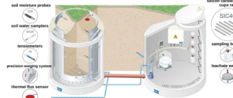
The lysimeters of the SoilCan network are arranged in hexagons of six lysimeters (consecutively indicated as L1, L2, ..., L6) at one plot. Figure 1 shows a schematic draw-ing of the lysimeter configuration. Each of the lysimeters has a circular surface area of 1 m2 and a depth of 1.5 m. The lysimeters are equipped with different sensors for measuring matric potential at 10, 30, 50 and 140 cm below the ground surface. The volumetric soil water content is measured with TDR (time-domain reflectometry) sensors at three different depths (10, 30, and 50 cm). Further measurements of CO2 concentration, soil heat flux and net radiation are conducted continuously. The matric potential at the lower boundary is controlled by a set of suction cups, such that water can be pumped into and out of the lysimeter. An automatic pump-ing system is used to adjust the pressure head at the lower boundary to the value of three reference tensiometers in-stalled in the field. The lysimeters are equipped with a weigh-ing system that allows for a resolution of 10 g (respectively 0.01 mm) for measuring the mass of the lysimeter and of 1 g for recording the mass of the seepage water reservoir. The mass data we refer to as raw data or signal were internally ac-quired at a frequency of 0.2 Hz (5 s), averaged with a moving mean over six of these 5 s values and logged with a frequency of one per minute.

At the research site in Bad Lauchstädt, three hexagons (here indicated as BL1, BL2, and BL3) with a total of 18 lysimeters were set up. Two hexagons (12 lysimeters) are cultivated with crops (BL1 and BL2). In the period of the pre-sented data set (1 March–31 May 2013), the grown crop was winter rape. The other 6 lysimeters are covered with grass. For each hexagon, the soils originate from two different lo-cations in Germany. Therefore, in Bad Lauchstädt, we can in-vestigate data from six different soil textures from six differ-ent locations, each location represdiffer-ented with a total of three lysimeters.

2.2 Comprehensive processing scheme for

high-precision lysimeter data – basic procedure Lysimeters are always directly exposed to environmental conditions and therefore prone to multiple error sources. The determination of an accurate time-resolved water balance re-quires an adequate data processing to eliminate these

influ-Figure 1. Schematic drawing of a lysimeter (left) as used in SoilCan attached to the central service pit (right).

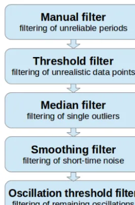
ences. We propose a processing scheme that should include five major steps (Fig. 2):

The threshold filter and the smoothing filter are described in detail by Schrader et al. (2013) and will therefore only be shortly addressed. To this basic scheme we added a man-ual filter, a median filter and an oscillation threshold filter as further components, which we consider to be essential for the determination of temporally highly resolved fluxes us-ing lysimeter data. It is important to conduct the filterus-ing in the suggested sequence. In particular, the filtering of discrete events (filter steps 1–3) has to be done prior to the filtering of noise (4–5). Otherwise, distinct events will be blurred by smoothing and cannot be filtered effectively afterwards.

Apart from the first filter step (manual filter), all the filter steps are applied to the mass data of the seepage water tank, corresponding to the seepage water flux, as well as to the summarized mass data of lysimeter and seepage water tank, corresponding to the flux at the soil–atmosphere interface (P

and ET). Only the manual filter is applied to the mass data sets of the seepage water tank and the lysimeter (before sum-marizing it). The threshold filter is first applied to the seepage mass data to eliminate possible spikes in the data (especially due to automatic emptying of the seepage water tank) before calculating the sum of lysimeter and seepage mass. In the following subsections, we will describe and discuss each of the individual filtering steps in detail.

2.2.1 Manual filter

pro-Figure 2. Flowchart of the basic processing scheme.

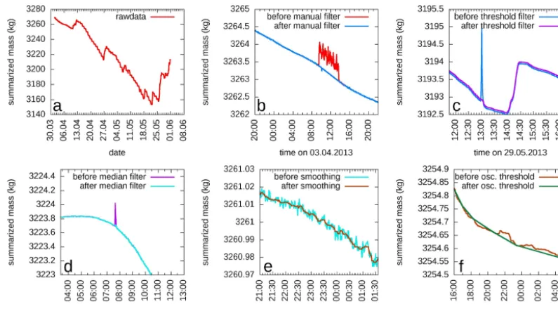
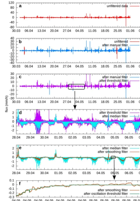
tocols of the technicians and the data transfer logs of the lysimeters, but this refers to other than mass data and is not within the scope of this study. Another option could be to determine heavily affected time periods by checking the au-tomatically processed results. In the presented data set, we exposed a manual filtering for some hours on three differ-ent days with known maintenance and at two further periods, where a single lysimeter showed distinct outliers in the data. During these periods, there was no precipitation detected by the nearby rain gauge and the weighing data were interpo-lated to fill the measurement gaps. The effect of the manual filter is illustrated in Fig. 3b compared to raw data (Fig. 3a). 2.2.2 Threshold filter

The threshold filter has the capability of removing strong and short external influences from the data set. Typical er-ror sources are mass changes during automatic emptying of the seepage water storage tanks, humans or (heavy) animals stepping on the lysimeter, or malfunctions in data transfer. By defining thresholds for the maximum possible precipita-tion, evapotranspiration and the maximum mass change in the seepage water reservoir, the filter can detect physically unrealistic fluxes. These data points are removed and substi-tuted by linear interpolations. Small errors, caused by wind effects or, for instance, by small animals, cannot properly be removed from the data at this stage because the filter thresh-old should not undershoot high but still reasonable water fluxes. The description of the parameter selection is given in Sect. 2.3.1. An example for the benefit of the threshold filter is illustrated in Fig. 3c.

2.2.3 Median filter

While the threshold filter is a suitable tool to eliminate large errors, influences, that lead to only small mass changes (like small animals, wind, temperature-effects, and signal noise) are not removed. The first step for a reduction of these er-rors is the application of a median filter that eliminates from the data set short-term spikes that are below the limits of the threshold filter. The effect of the median filter is illustrated in Fig. 3d. This filter is a very effective amendment to the threshold filter for eliminating discrete errors. As described in Sect. 2.3.1 we use a time window of 15 min for the calcu-lation of the median.

2.2.4 Smoothing filter

While the previous filter steps are designed to eliminate dis-crete errors, the last two filter steps are designed to deal with remaining diffuse noise. The primary step in removing noise is a smoothing filter, where different smoothing algorithms can be used. Schrader et al. (2013) discussed the application of a second-degree Savitzky–Golay filter (which is based on a polynomial approximation) as well as the simple moving average, both of which show different advantages and dis-advantages for the application of lysimeter data. The overall issue of such smoothing filters is the blurring of short time effects and the mixing of ET andP. To avoid temporal dis-tortion or even elimination of short-term events, it is advis-able to restrict smoothing to a short time period. In our cal-culations, we used the simple moving average with a time window ofn=15 min, to restore a high temporal resolution and to avoid distinct blurring effects (see Sect. 2.3.1). The moving average calculates the arithmetic mean of the data points in the time window fromti−(n−1)/2 toti+(n−1)/2 for each data point at timeti. Figure 3e gives an illustration of

the effect of the smoothing filter.

2.2.5 Oscillation threshold filter

Smoothing filters are not able to eliminate all fluctuations, especially when they are limited to short time windows to retain a high temporal resolution and to preserve short-term effects. In situations where the external forcing (precipitation or evapotranspiration) is low or vanishing, remaining noise will alter the calculated fluxes. Figure 3f illustrates the is-sue of remaining noise components in the calculated fluxes before and after the use of the oscillation threshold filter. Al-though the oscillatory fluxes are small, they may lead to no-ticeable deviations in the cumulative values of precipitation and evapotranspiration.

Figure 3. Examples for the effect of the different filtering steps on the mass data (here: summarized mass of lysimeter and seepage water tank of lysimeter BL1-L1). Please note the different scaling of theyaxes. (a) raw data, (b) manual filter, (c) threshold filter, (d) median filter, (e) smoothing filter, (f) oscillation threshold filter.

this problem, our algorithm ensures that also slow processes will be recognized as long as their contribution in a sum exceeds the defined threshold. Starting from an initial data point, this algorithm determines the next point in time where the cumulative mass change exceeds a predefined threshold. When this threshold is reached, the intermediate data points are linearly interpolated:

Mk=Mi+

Ml−Mi

tl−ti

·(tk−ti) , for i < k < l−1. (1)

In this formula,Mis the sum of the masses of the lysimeter and the seepage water tank at timet,kindicates the starting point, andlthe first point where the threshold has been ex-ceeded. Small fluctuations that are not due to real fluxes are eliminated. The oscillation threshold filter enables the reg-istration of slow processes such as light rain events, snow-fall, or evapotranspiration if they are lasting long enough to exceed the threshold as a sum. The functioning of this algo-rithm is illustrated in Fig. 3f. Nevertheless, processes with a low flux rate and a short duration – such that the threshold is not reached – are still not registered and they fall out of the precision range defined by the oscillation threshold. Thus, the threshold value defines the limit of processes that cannot fur-ther be resolved because they cannot be distinguished from the remaining noise. The choice of the oscillation threshold value is discussed in Sect. 2.3.1.

2.2.6 Calculation of fluxes

After the execution of the presented filtering steps, the fluxes can be calculated from the processed data set. The seepage

fluxSis simply calculated from the increase in the massmS of the seepage water reservoir.

S(ti)=

mS(ti+1)−mS(ti)

ti+1−ti

(2) The calculation of precipitation and evapotranspiration re-quires a distinction of these cases. This separation implies the assumption that no evapotranspiration is occurring during rainfall events or that evapotranspiration is at least negligible.

J (ti)=

Mi+1−Mi

ti+1−ti

(3)

P (ti)= (

J (ti), if J (ti)>=0

0, if J (ti) <0

(4)

ET(t )= (

0, if J (ti)>=0 −J (ti), if J (ti) <0

(5)

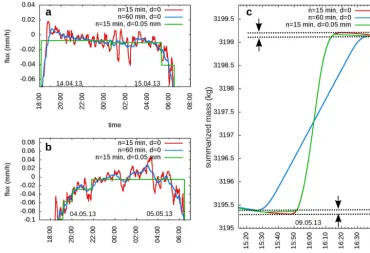
Figure 4. Effects of different averaging time windowsnand the oscillation thresholddon the data oscillations (noise error) during nighttime situations (a, b) and the underestimation of precipitation due to the mixing of ET andP(mixing error) during a precipitation event (c). While (a) and (b) show the calculated fluxes, (c) shows the summarized mass of lysimeter and seepage water representing the cumulative flux at the upper boundary. The underestimation of the precipitation-induced mass change in (c) due to the 60 min smoothing is indicated in the figure.

2.3 Filter parameter selection and adaptive methods 2.3.1 Filter parameter selection

The basic processing scheme provides all the necessary com-ponents to tackle the different error sources on the lysimeter weighing data and to obtain a time-resolved water balance. However, the operator has to define some parameters, which influence the quality of the filtering and the precision of the resulting fluxes. The choice of the threshold values in filter-ing step 2 (threshold filter) is rather simple and can be de-termined by the maximal pumping rate at the lower bound-ary of the lysimeter, the maximal precipitation rate and the maximal ET rate, including a safety factor (see also Schrader et al., 2013). The parameters that were used as standard in our calculations are listed in Table 1.

The selection of the time window for the median and the smoothing filter (filter steps 3 and 4) is much more critical. While large time windows ensure an effective reduction of noise (noise error), such large averaging times also reduce the temporal resolution of processes and lead to a progressive mixing of P and ET (mixing error), which is also an error source in the calculation of an accurate water balance. The influence of the smoothing filter and the oscillation threshold filter on the noise error and the mixing error is displayed in Fig. 4. By using the subsequent oscillation threshold filter, it is possible to shorten time periods for averaging and to retain

Table 1. Parameters for the different filters in the basic process-ing approach that were used as standard. If no other information is given, the calculations refer to these parameters.

Standard parameters for the basic processing approach

threshold for lysimeter mass changes ±60 mm h−1 threshold for seepage mass changes ±9 mm h−1

median filter window 15 min

smoothing filter window 15 min

oscillation threshold 50 g

a higher resolution of processes. Considering the high dy-namics of observed precipitation events of less than 20 min in periods of high evapotranspiration (i.e., short summer rain; see also examples in Fig. 7) we recommend a time window of 15 min at maximum, which is used in our calculations. This ensures keeping a high temporal resolution of our processed data set. This window length of 15 min is also sufficient for the purposes of the median filter, which is designed to elim-inate local errors of only some data points in the data and is also used for our calculations.

fluxes. Figure 4a and b illustrate that a very effective elim-ination of noise is possible, using the oscillation threshold filter. Figure 4c further shows that the combination of the short time smoothing together with the oscillation threshold filter leads to a better temporal reflection of the precipitation process compared to the removal of oscillations by the use of a longer averaging time. However, it can be seen that the oscillation threshold filter also leads to an underestimation of precipitation events, comparable to the described mixing error.

Higher oscillation thresholds increase the risk of filtering oscillations that represent real processes (e.g., dew forma-tion). The threshold has to be chosen as large as necessary (to filter noise) and as small as possible (to retain slow pro-cesses and to prevent the underestimation during rain events). This idea is reflected by the subsequently described adaptive methods, attempting to optimize this parameter with respect to signal. In addition to the use of these techniques, we ap-plied the oscillation threshold filter to derive a possible range for the cumulative water balance by selecting a maximum and a minimum value for the possible threshold. As mini-mum value we used a threshold of 0 g, implying that every remaining oscillation is interpreted as real effects. To deter-mine a maximum threshold, we investigated the fluxes of the different lysimeters during nighttime conditions and selected the threshold at a height where nearly all of these night-time oscillations vanished. For our data set, we ended with a maximum value of 50 g. This implies that for the maximum threshold, only processes which contribute with a minimum of 0.05 mm to the cumulative flux are considered in the water balance. While the use of the minimum threshold will lead to an overestimation of the cumulative fluxes ofP and ET, the use of the maximum threshold will cause an underestimation of these values. We therefore assume to find the true values in between these limits.

2.3.2 Parameter adaptation using an estimate of the signal strength

Peters et al. (2014) suggest to adapt the parameters for the smoothing window length and the oscillation threshold to the signal strength in the data. The idea behind this method is to increase the smoothing time window and the oscillation threshold in periods where the signal strength is low and the noise is becoming more dominant and to reduce them in sit-uations where noise is less relevant. In their AWAT filter al-gorithm, Peters et al. (2014) estimate the signal strength by applying a polynomial fit to the data within a predefined time window. The deviation of the data to the polynomial fit leads to a measure of the signal strength. This estimate is used to adapt the time window for smoothing as well as the oscil-lation threshold to the signal strength. The parameters are varied in a range between a minimum and a maximum value, predefined by the operator. For the oscillation threshold, Pe-ters et al. (2014) suggested to choose the maximal resolution

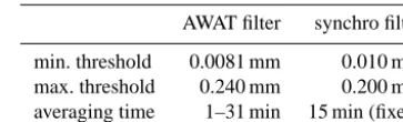
Table 2. Parameters used for the adaptive methods.

AWAT filter synchro filter

min. threshold 0.0081 mm 0.010 mm max. threshold 0.240 mm 0.200 mm averaging time 1–31 min 15 min (fixed)

of the weighing system as minimum value. For our data set, we chose a minimum value of 10 g (respectively 0.01 mm). The further values applied for the AWAT filter are listed in Table 2 together with the parameters applied in the filtering approach using parallel lysimeters as described in Sect. 2.3.3.

2.3.3 Parameter adaptation using parallel lysimeters

3 Results and discussion 3.1 Flux dynamics

The influence of the different processing steps on the calcu-lated fluxes for one example lysimeter is illustrated in Fig. 5. While the manual filter and the threshold filter succeed in eliminating large erroneous fluxes (Fig. 5b, c), the subse-quent processing steps (Fig. 5d–f) lead to a pronounced re-duction of small errors and noise. Because the filtering steps work on different scales, we zoom into the data for a good illustration of the effects.

To examine the remaining variability between the lysime-ters after the data processing, we compared the calculated precipitation fluxes for the different lysimeters at our re-search site . As a first part of that comparison, the mean and the range of the calculated fluxes across the soil–atmosphere interface of all 12 crop lysimeters have been calculated (we omitted the grass lysimeters in this consideration because of the different transpiration). The good accordance is il-lustrated in Fig. 6. The highest variation with a range of 4 mm h−1corresponds to the event with the maximum pre-cipitation rate of 20.2 mm h−1.

3.2 Temporal resolution

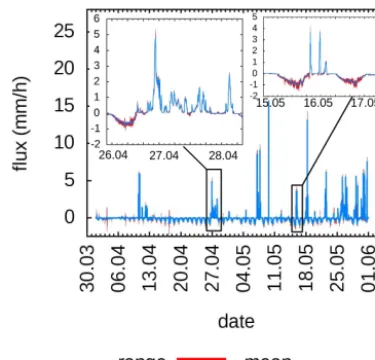
The ability of preserving detailed dynamics and a good tem-poral resolution by using the basic filtering scheme becomes obvious when looking at the calculated fluxes. Figure 7a shows a heavy rainfall event on 9 May 2013 with a dura-tion of only about 20 min, which would be spread out to a moderate rainfall by applying larger averaging times. A light and short rainfall on 4 May 2013 between situations of evap-otranspiration is displayed in Fig. 7b. Larger averaging times would lead to a merging of ET fluxes and precipitation fluxes. Finally, Fig. 7c and d illustrate the intense dynamics of pre-cipitation events in the examples of a medium rainfall event in the period from 26 to 28 April 2013 and a light rainfall from 12 April 2013. A large part of this dynamics would be blurred with an averaging time of more than 1 h.

3.3 Cumulative precipitation

For investigating the accuracy of the determined fluxes, the cumulative precipitation for all 18 lysimeters at the Bad Lauchstädt site was calculated for the minimal and the maxi-mal oscillation threshold. The range between the mean values for these two cases was plotted together with the measure-ment of the nearby rain gauge (Fig. 8). The indicated filter uncertainty is representing the range of uncertainty, which results from the contrary influences of noise error and mix-ing error, and was calculated by usmix-ing the minimal and max-imal threshold as described in Sect. 2.3.1. This consideration leaves us at the end of the data time series with a cumula-tive precipitation of 158.2±3.2 mm, indicating a remaining uncertainty of only 2 %. Besides the filtering uncertainty, the

Figure 5. Effect of the different processing steps on the calculated fluxes at the soil–atmosphere interface for one exemplary lysimeter (BL1-L1). After presenting the unfiltered data (a), the effect of the manual filter (b), the threshold filter (c), the median filter (d), the smoothing filter (e) and the oscillation threshold filter (f) is shown. For (d), (e) and (f), zoom levels were increased to illustrate the dif-ferent scales affected by the filtering steps. Please note the difdif-ferent scaling of the axes.

Figure 6. Variations in the calculated fluxes between the different crop lysimeters. The area in red shows the range of minimal and maximal calculations.

Figure 7. Short time dynamics of precipitation events for selected rain events of 9 May 2013 (a), 4 May 2013 (b), 26–28 April 2013 (c) and 12 April 2013 (d).

series. These lower values can be caused by the known errors of the Hellmann rain gauge system (e.g., Richter, 1995) or by the heterogeneity of the rainfalls and the distance between the measurement devices. Figure 8b shows a comparison of the precipitation on a daily basis.

Figure 9 shows the filter uncertainty together with the re-sults for the adaptive and the basic approach using differ-ent parameter selections. In all the approaches, the data were processed with the first three filtering steps (manual filter, threshold filter, median filter) before doing further filtering steps. In the case of an averaging time of 5 min, we also re-duced the time window for the median filter to 5 min. Only the approaches with a more extreme choice of the filtering

Figure 8. The calculated precipitation with its uncertainties as cu-mulative precipitation (a) and daily precipitation (b). The total un-certainty is the sum of the estimated filtering unun-certainty and the standard deviation of the different measurements on the 18 lysime-ters.

Figure 9. The values for cumulative precipitation together with the standard deviation regarding the measurements of the 18 different lysimeters for different parameter selections and the two adaptive methods.

the uncertainty range. The difference of the basic approach to the adaptive methods is therefore quite low and does not exceed the 2 % uncertainty. However, this may be due to the fact that the positive effect of remaining noise is compen-sated partly by a negative effect of the mixing error. If this would be the reason, an underestimation of precipitation dur-ing events would go in hand with an overestimation of pre-cipitation during situations of low external forcing. Such a behavior would lead to deviations in the time-resolved fluxes, even if these errors would cancel out in the cumulative bal-ance.

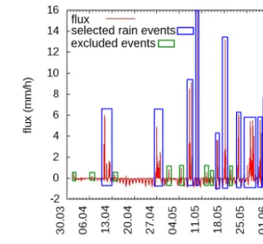
To further examine if the more sophisticated filtering ap-proaches (the AWAT filter, and the synchro filter) lead to a re-duction of both these error components and therefore to a bet-ter accuracy of the calculated wabet-ter balance over the whole time series, a partitioning of the data set into periods with and without precipitation was done. Figure 10 shows the differ-ent periods. Rainfalls with a minimum flux rate of 1 mm h−1 (blue boxes) were chosen such that the selected period starts and ends between 200 and 250 min before and after the regis-tration of positive fluxes. This is to ensure that even the tem-poral blurring of high averaging times of 180 min will not lead to a spreading out of the fluxes of the selected time win-dow. In these periods of distinct rain, the noise error plays a minor role (because the fluxes are mainly positive and do not oscillate from positive to negative values) and so they can be used to estimate the size of the mixing error. The green boxes indicate very small rainfalls. These periods were ex-cluded from the examination because, in such cases, the mix-ing error as well as the noise error are relevant. The rest of the data set represents periods of dominant noise and minor error. The only contributions to precipitation are very small processes like dew formation.

For estimating the contribution of the investigated er-rors we compared the calculated precipitation to a reference value. For the rain periods, where noise is playing a minor role, we used the basic approach with an oscillation thresh-old of 10 g (corresponding to the weighing accuracy) as refer-ence. This low value prevents distinct influences of the mix-ing errors, while the noise effect is assumed to be minor. For the no-rain periods, where the mixing of ET andPis less im-portant, we used the basic approach with the maximum oscil-lation threshold value of 50 g as reference, where nearly all oscillation during nighttime vanished. Figure 11a shows the deviations to these reference values for different averaging times, without applying an oscillation threshold filter. The deviation during the rain periods, indicated by the blue line, is an estimate for the mixing error, the deviation during the no-rain periods (red line) is an estimate for the noise error. The noise error is clearly decreasing with increasing averag-ing time, while the contribution of the mixaverag-ing error is increas-ing. For an averaging time of about 50 min, the two errors are compensating each other. For higher averaging times, the mixing error is increasing and leads to a deviation of about 5 mm for an averaging time of 120 min. Averaging time

be-Figure 10. Selection of periods for the investigation of the noise and the mixing error. The purple periods were selected for the estimation of the mixing error, the blue periods of light rain were excluded because of the contribution to both errors, and the rest of the data set was used for the estimation of the noise error.

Figure 11. Effects of averaging time (a) and oscillation threshold value (b) on the estimates for the mixing error and the noise error. The error estimates of the AWAT filter and the synchro filter are indicated in panel (a) with green stars for the AWAT filter and purple stars for the synchro filter.

low 20 min (without the use of an oscillation threshold) leads to a strong increase of the noise error.

higher temporal resolution (for a better reflection of the pro-cess dynamics) and the possibility to get an estimation of the filtering uncertainty in the previously described way. Reca-pitulating these results, the overall error occurring from the described filtering errors, excluding averaging times below half an hour without using an oscillation threshold filter, con-tribute to the total water balance with a maximum of about 3 % (for the AWAT filter and the synchro filter). The result-ing error estimates are both indicated in Fig. 11a. Both meth-ods further reduce the errors compared to the range of errors given by the accuracy range and, hence, provide a better es-timate. While the estimate for the noise error is less for the synchro filter (1.1 mm) than for the AWAT filter (2.2 mm), the AWAT filter is more effective in avoiding the mixing er-ror during rain periods (0.2 mm AWAT,−1.0 mm synchro). Here it has to be stated that our reference value is only an estimator for the real value, and the real value for the cumu-lative precipitation is not known exactly. This is especially important when interpreting the results for the noise error, where some real effects might be misinterpreted as errors. In summary, the adaptive methods seem to achieve a good reduction of the filtering errors for our test data set, but the advantage in comparison to the basic methods seems to be minor. This is especially the case if we compare the errors to the higher variability between the different lysimeter mea-surements, which is not dependent on the filter method. Nev-ertheless, the filtering errors in other data sets may be higher because of a greater influence of noise on the data. We there-fore recommend to always estimate the uncertainty in the de-scribed way by choosing a minimum and a maximum thresh-old for getting an idea of the possible filtering uncertainty. If this uncertainty range is relatively high, it may be worth to use more sophisticated methods like the AWAT filter or – provided several parallel lysimeters are available – the syn-chro filter to further reduce the uncertainty.

3.4 Cumulative evapotranspiration

The influence of the filtering error discussed in the previous chapter for the cumulative precipitation is similar for the cu-mulative evapotranspiration. An overestimation ofP (posi-tive flux) comes along with an overestimation of ET (neg-ative flux), because the total flux at the upper boundary is determined by the absolute mass change of the lysimeter and the seepage water reservoir. Thus, an absolute uncertainty of 3 mm for the cumulative value of P due to filtering uncer-tainty implies the same unceruncer-tainty for ET. The relative un-certainty depends on the absolute value of ET. For the used data sets, the absolute value of ET exceeded the value ofP, so that the described filtering uncertainty is even below the value of 2 %.

However, the variance between the different lysimeter measurements is much higher for ET than for precipitation. In Fig. 12 it is illustrated as mean and standard deviation for the basic processing approach with an oscillation

thresh-Figure 12. Cumulative evapotranspiration (mean±standard devia-tion) for the 12 crop lysimeters of the Bad Lauchstädt test site. The small picture shows the results separated in soil type groups.

old of 50 g. For this calculation, only the 12 crop lysime-ters of the Bad Lauchstädt test site were taken into account, the 6 grassland lysimeters were excluded because of the dif-ferent transpiration. The resulting standard deviation at the end of the time series is only about 6.5 % of the total. The higher variance may be caused by differences in plant growth as well as by differences in soil properties. This uncertainty (together with the filter uncertainty about 8.5 %) can serve as a first estimate for the uncertainty when using lysime-ter measurements for estimating ET for a surrounding field of the same soil and vegetation. This implies the assump-tion that the plant development on the lysimeters reflects the plant development in the field at least in the mean, without systematic deviations. To investigate the influence of the soil type, the small figures show the cumulative ET separated by the soil origin. Two soils (Sauerbach and Bad Lauchstädt) exhibit considerable differences in the mean evapotranspira-tion and a reduced variability. Because of the small data basis with only three replicates per soil, we refrain from a statisti-cal examination of the influence of the soil type.

3.5 Seepage flux

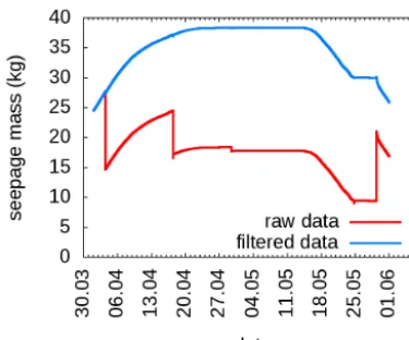
Figure 13. Comparison of processed and raw seepage mass data for the lysimeter BL2-L1.

on the detailed control of the pumps at the lower boundary which add or remove water to or from the lysimeter to adjust the matric potential at the lower boundary of the lysimeter in accordance with the field measurements.

3.6 Representativeness of evaluated time interval For the evaluation of the proposed filtering scheme we used data from a rather short time interval of only 2 months, so one may question its representativeness. For discussing the effects of the various filtering steps on the data we need to look at them at very high temporal resolution. A longer data set would have hidden the details of the filtering effects. Oc-casions where our filtering scheme could run into problems are dates where extensive soil management (e.g., sowing, harvesting of crops, and tillage), which disturbs the weigh-ing data, is conducted on the lysimeters. On these dates, the manual filtering would have to be done very properly before the automatic filtering routines could be applied. Other pe-riods that might be challenging to handle are pepe-riods where the lysimeters are covered with snow, since the snow cover on the lysimeter is often connected to the snow cover outside the lysimeters which, in turn, heavily disturbs the weighing data. This, however, is a well-known problem in lysimetry which by nature produces unreliable weighing data that also need to be corrected manually in the data set. Here, of course, additional information about the site conditions (snow cover) during winter is required. All other situations should be well evaluated with the current filtering scheme.

4 Summary and conclusions

In this study, we presented a basic filtering scheme to re-move the various kinds of errors on the lysimeter weighing data, leading to a falsification of the calculated water bal-ance components. We showed the effectivity of these filter components and investigated the influence of the

parame-ter selection on the accuracy of the calculated waparame-ter balance components. Furthermore, we used the data set of 18 parallel running lysimeters to determine the variability between these measurements and compared it with the filtering uncertainty. For our test data set, we found that the uncertainty in the cumulative precipitation and evapotranspiration due to the choice of the filtering parameters for noise reduction is only about 2 %. This uncertainty is less than the uncertainty that is given by the heterogeneity of the precipitation measurements between the different lysimeters, which is 2.7 %. For the use of lysimeter measurements to estimate precipitation in the surrounding field, both uncertainties have to be summed up, which makes a total uncertainty of approximately 5 %. This accuracy can be achieved while maintaining a high tempo-ral resolution of 15 min. Examples were shown where good temporal resolution is necessary to retain the correct process dynamics. Despite the higher variability in the resulting ET (6.5 %), which may be due to differences in plant growth, this moderate uncertainty below 10 % (after adding both er-rors) shows the potential of using lysimeter measurements as a suitable estimate of field ET with a tolerable uncertainty (what should be investigated in further studies). We further tested two filtering approaches, where the filtering parame-ters are adapted to additional data. Both adaptive methods, the AWAT filter (Peters et al., 2014) and the synchro fil-ter, showed a good reduction of noise within the uncertainty limits. By using subsets of the data, we further investigated the dependency of the filtering errors on averaging time and oscillation threshold. We showed that the use of averaging times between approximately 30 min and 1 h lead to the low-est filtering errors. However, using a combination of a short smoothing time (15 min) together with the oscillation thresh-old filter, the filtering error could even be further reduced. The AWAT filter and the synchro filter both showed a good reduction of both error components. However, the improve-ment of these methods compared to the basic approach with adequate filtering parameters was only minor.

The Supplement related to this article is available online at doi:10.5194/hess-19-3405-2015-supplement.

U. Franko for the measurements of the rain gauge. We also thank our partners from UMS GmbH, Munich, for their support by solving technical problems. We further thank the Arbeitskreis Lysimeterdatenauswertung for the fruitful discussions.

The article processing charges for this open-access publication were covered by a Research

Centre of the Helmholtz Association.

Edited by: A. Loew

References

Bogena, H., Schulz, K., and Vereecken, H.: Towards a network of observatories in terrestrial environmental research, Adv. Geosci., 9, 109–114, doi:10.5194/adgeo-9-109-2006, 2006.

Evett, S., Schwartz, R., Howell, T., Baumhardt, R., and Copeland, K.: Can weighing lysimeter ET represent surround-ing field ET well enough to test flux station measurements of daily and sub-daily ET?, Adv. Water Resour., 50, 79–90, doi:10.1016/j.advwatres.2012.07.023, 2012.

Fank, J.: Wasserbilanzauswertung aus Präzisionslysimeterdaten, in: Proceedings 15. Gumpensteiner Lysimetertagung, Irdning, Austria, 16–17 April 2013, 85–92, available at: http://www. raumberg-gumpenstein.at/cm4/de/forschung/publikationen/ downloadsveranstaltungen/finish/742-lysimetertagung-2013/ 11981-wasserbilanzauswertung-aus-praezisionslysimeterdaten. html (last access: 3 August 2015), 2013.

Fank, J. and von Unold, G.: High-precision weighable field Lysimeter–a tool to measure water and solute balance parame-ters, International Water and Irrigation, 27, 28–32, 2007. Gebler, S., Hendricks Franssen, H.-J., Pütz, T., Post, H., Schmidt,

M., and Vereecken, H.: Actual evapotranspiration and precipi-tation measured by lysimeters: a comparison with eddy covari-ance and tipping bucket, Hydrol. Earth Syst. Sci., 19, 2145–2161, doi:10.5194/hess-19-2145-2015, 2015.

Goss, M. and Ehlers, W.: The role of lysimeters in the de-velopment of our understanding of soil water and nutrient dynamics in ecosystems, Soil Use Manage., 25, 213–223, doi:10.1111/j.1475-2743.2009.00230.x, 2009.

Howell, T., Schneider, A., and Jensen, M.: History of lysimeter de-sign and use for evapotranspiration measurements, in: Lysimeters for Evapotranspiration and Environmental Measurements, edited by: Allen, R., Howell, T., Pruitt, W., Walter, I., and Jensen, M., Proc. Intl. Symp. Lysimetry, Reston, VA, 1–9, ASCE, 1991. Howell, T., Schneider, A., Dusek, D., Marek, T., and Steiner, J.:

Cal-ibration and scale performance of bushland weighing lysimeters, Trans. ASAE, 38, 1019–1024, 1995.

Lanthaler, C. and Fank, J.: Lysimeter stations and soil hydrology measuring sites in Europe – Results of a 2004 survey, in: Proceedings 11. Gumpensteiner Lysimetertagung, Irdning, Austria, 5 and 6 April 2005, 19–24, available at: http://www. raumberg-gumpenstein.at/cm4/de/forschung/publikationen/ downloadsveranstaltungen/finish/69-lysimetertagung-2005/ 772-lysimeter-stations-and-soil-hydrology-measuring-sites.htm (last access: 3 August 2015), 2005.

Loos, C., Gayler, S., and Priesack, E.: Assessment of water balance simulations for large-scale weighing lysimters, J. Hydrol., 335, 259–270, doi:10.1016/j.jhydrol.2006.11.017, 2007.

Meissner, R., Seeger, J., Rupp, H., Seyfarth, M., and Borg, H.: Mea-surement of dew, fog, and rime with a high-precision gravitation lysimeter, J. Plant Nutr. Soil Sci., 170, 335–344, 2007.

Nolz, R., Kammerer, G., and Cepuder, P.: Interpretation of lysime-ter weighing data affected by wind, J. Plant Nutr. Soil Sci., 176, 200–208, 2013a.

Nolz, R., Kammerer, G., and Cepuder, P.: Verbesserung der Auswertung von Lysimeter-Wiegedaten, Die Bodenkultur, Jour-nal for Land Management, Food and Environment, 64, 27–35, 2013b.

Nolz, R., Cepuder, P., and Kammerer, G.: Determining soil water-balance components using an irrigated grass lysimeter in NE Austria, J. Plant Nutr. Soil Sci., 177, 237–244, 2014.

Peters, A., Nehls, T., Schonsky, H., and Wessolek, G.: Separating precipitation and evapotranspiration from noise – a new filter routine for high-resolution lysimeter data, Hydrol. Earth Syst. Sci., 18, 1189–1198, doi:10.5194/hess-18-1189-2014, 2014. Pütz, T., Kiese, R., Zacharias, S., Bogena, H., Priesack, E.,

Wollschläger, U., Schwank, M., Papen, H., von Unold, G., and Vereecken, H.: TERENO-SOILCan – Ein Lysimeter Netzwerk in Deutschland, in: 14. Gumpensteiner Lysimetertagung 2011, Irdning, Austria, 3–4 May 2011, 5–10, available at: http://www. raumberg-gumpenstein.at/cm4/de/forschung/publikationen/ downloadsveranstaltungen/finish/514-lysimetertagung-2011/ 4352-tereno-soilcan-ein-lysimeter-netzwerk-in-deutschland. html (last access: 3 August 2015), 2011.

Richter, D.: Ergebnisse methodischer Untersuchungen zur Korrektur des systematischen Messfehlers des Hellmann-Niederschlagsmessers, vol. 94, Deutscher Wetterdienst, Offenbach, Germany, 1995.

Schrader, F., Durner, W., Fank, J., Gebler, S., Pütz, T., Hannes, M., and Wollschläger, U.: Estimating precipitation and actual evap-otranspiration from precision lysimeter measurements, Procedia Environmental Sciences, 19, 543–552, 2013.

Seneviratne, S., Lehner, I., Gurtz, J., Teuling, A., Lang, H., Moser, U., Grebner, D., Menzel, L., Schroff, K., Vitvar, T., and Zappa, M.: Swiss prealpine Rietholzbach research catchment and lysimeter: 32 year time series and 2003 drought event, Water Re-sour. Res., 48, W06526, doi:10.1029/2011WR011749, 2012. Shuttleworth, W.: Terrestrial Hydrometeorology, John Wiley &

Sons, Ltd, Chichester, West Sussex, UK, 2012.

Teuling, A., Hirschi, M., Ohmura, A., Wild, M., Reichstein, M., Ciais, P., Buchmann, N., Ammann, C., Montagnani, L., Richard-son, A., Wohlfahrt, G., and Seneviratne, S.: A regional perspec-tive on trends in continental evaporation, Geophys. Res. Let., 36, L02404, doi:10.1029/2008GL036584, 2009.

van Bavel, C.: Lysimetric measurements of evapotranspiration rates in the eastern United States, Soil Sci. Soc. Am. Proc., 25, 138– 141, 1961.

Vaughan, P., Trout, T., and Ayars, J.: A processing method for weighing lysimeter data and comparison to micrometeorological ETo predictions, Agr. Water Manage., 88, 141–146, 2007. Vaughan, P. J. and Ayars, J. E.: Noise reduction methods for

Yang, J., Li, B., and Liu, S.: A large weighing lysimeter for evap-otranspiration and soilwater–groundwater exchange studies, Hy-drol. Process., 14, 1887–1897, 2000.

Young, M., Wierenga, P., and Mancino, C.: Large weighing lysime-ters for water use and deep percolation studies, Soil Sci., 161, 491–501, 1996.