A nonparametric statistical technique for combining global precipitation datasets: development and hydrological evaluation over the Iberian Peninsula

https://doi.org/10.5194/hess-22-1371-2018 © Author(s) 2018. This work is distributed under the Creative Commons Attribution 3.0 License.

A nonparametric statistical technique for combining global

precipitation datasets: development and hydrological

evaluation over the Iberian Peninsula

Md Abul Ehsan Bhuiyan1, Efthymios I. Nikolopoulos1,2, Emmanouil N. Anagnostou1, Pere Quintana-Seguí3, and Anaïs Barella-Ortiz3,4

1_{Department of Civil and Environmental Engineering, University of Connecticut, Storrs, CT, USA} 2_{Innovative Technologies Center S.A., Athens, Greece}

3_{Ebro Observatory, Ramon Llull University – CSIC, Roquetes (Tarragona), Spain} 4_{Castilla-La Mancha University, Toledo, Spain}

Correspondence:Emmanouil N. Anagnostou ([email protected]) Received: 6 May 2017 – Discussion started: 6 June 2017

Revised: 16 November 2017 – Accepted: 10 January 2018 – Published: 26 February 2018

Abstract. This study investigates the use of a nonparamet-ric, tree-based model, quantile regression forests (QRF), for combining multiple global precipitation datasets and charac-terizing the uncertainty of the combined product. We used the Iberian Peninsula as the study area, with a study period spanning 11 years (2000–2010). Inputs to the QRF model included three satellite precipitation products, CMORPH, PERSIANN, and 3B42 (V7); an atmospheric reanalysis pre-cipitation and air temperature dataset; satellite-derived near-surface daily soil moisture data; and a terrain elevation dataset. We calibrated the QRF model for two seasons and two terrain elevation categories and used it to generate en-semble for these conditions. Evaluation of the combined product was based on a high-resolution, ground-reference precipitation dataset (SAFRAN) available at 5 km 1 h−1 res-olution. Furthermore, to evaluate relative improvements and the overall impact of the combined product in hydrolog-ical response, we used the generated ensemble to force a distributed hydrological model (the SURFEX land surface model and the RAPID river routing scheme) and compared its streamflow simulation results with the corresponding sim-ulations from the individual global precipitation and refer-ence datasets. We concluded that the proposed technique could generate realizations that successfully encapsulate the reference precipitation and provide significant improvement in streamflow simulations, with reduction in systematic and random error on the order of 20–99 and 44–88 %, respec-tively, when considering the ensemble mean.

1 Introduction

Accurate estimates of precipitation on a global scale, which are essential to hydrometeorological applications (Stephens and Kummerow, 2007), rely primarily on satellite-based ob-servations and atmospheric reanalysis simulations. Although advancement in both satellite retrievals and reanalysis-based precipitation datasets has been continuous (Seyyedi et al., 2014; Dee et al., 2011; Huffman et al., 2007; Mo et al., 2012), they are still associated with several sources of er-ror (Derin et al., 2016; Mei et al., 2014; Seyyedi et al., 2014; Gottschalck et al., 2005; Peña-Arancibia et al., 2013) that limit their use in water resource applications. Quantifying and correcting the sources of the error and characterizing its propagation are important for improving and promoting the use of satellite and reanalysis precipitation estimates in hy-drological applications on a global scale.

depen-dencies (Hossain and Anagnostou, 2006; Teo and Grimes, 2007; Maggioni et al., 2014; Adler et al., 2001; AghaK-ouchak et al., 2009) and have used stochastically generated ensemble rainfall fields as input in hydrological models to study the satellite precipitation uncertainty propagation in the simulation of various hydrological variables. The two-dimensional satellite rainfall error model, SREM2-D (Hos-sain et al., 2006), has been used to evaluate the significance of surface soil moisture (Seyyedi et al., 2014) and seasonal-ity (Maggioni et al., 2017) in modeling the error structure of satellite rainfall products.

Given the multidimensionality of error dependence and the lack of a clear winner among the various precipitation datasets established by these studies, we argue that, to mit-igate the errors and uncertainties, one should combine the different precipitation datasets, taking into account the differ-ent climatological and land surface factors. A promising ap-proach to modeling appears to be the application of statistical nonparametric techniques, which efficiently combine infor-mation on several factors (Ciach et al., 2007; Gebremichael et al., 2011). In fact, although nonparametric statistical tech-niques are not widely used in rainfall estimation, some no-table examples exist in the literature, with encouraging re-sults. Ciach et al. (2007) established a nonparametric estima-tion technique based on weather radar data to characterize the uncertainties in radar precipitation estimates as a function of range, temporal scale, and season. Lakhankar et al. (2009) in-troduced a nonparametric technique to retrieve soil moisture from satellite remote sensing products in reliable ways with sufficient accuracy. Moreover, Gebremichael et al. (2011) de-veloped a nonparametric technique for satellite rainfall er-ror modeling using rain-gauge-adjusted, ground-based radar rainfall and reported improved satellite precipitation perfor-mance with relatively large variation at low and high rainfall rates.

The use of nonparametric statistical techniques in error modeling has also gained popularity in weather forecasting, climate change prediction, and the modeling of hydrologi-cal processes (Croley, 2003; Brown et al., 2010; Mujumdar et al., 2008; Yenigun et al., 2013). Recently, a wide variety of nonparametric techniques have been developed for error ana-lytics (Taillardat et al., 2016; He et al., 2017). Nonparametric statistical techniques require fewer assumptions for the form of the relationship and data. The advantages over parametric techniques for prediction are explained in detail in Guikema et al. (2010). Specifically, the authors exhibited better re-sults (lower prediction error) with nonparametric techniques than with parametric analysis models. The techniques they used were classification and regression trees (CART) and Bayesian additive regression trees (BART) (Chipman et al., 2010). Another nonparametric technique, random forest (RF) regression, which provides information about the full con-ditional distribution of the response variable, was used by Breiman (2001) and found to yield more robust predictions by stretching the use of the training data partition.

This paper investigates the use of a nonparametric statis-tical technique for optimally combining globally available precipitation sources from satellite and reanalysis products. Specifically, we use the quantile regression forests (QRF) tree-based regression model (Meinshausen, 2006) to com-bine dynamic (for example, temperature and soil moisture) and static (for example, elevation) land surface variables with multiple global precipitation sources to stochastically gener-ate improved precipitation ensemble. The proposed frame-work provides a consistent formalism for optimally combin-ing several rainfall products by uscombin-ing information from these datasets. It is, furthermore, able to characterize uncertainty through the ensemble representation of the combined pre-cipitation product. We present the development of the pro-posed framework and evaluate relative improvements in the combined rainfall product in detail. We also evaluate the new combined product in terms of hydrological simulations to as-sess the importance of precipitation improvement for stream-flow simulations, thus highlighting the usefulness of this ap-proach for global hydrological applications.

The paper is structured as follows: Sect. 2 briefly explains the study area and the datasets used. Section 3 describes the QRF model, the rainfall error analysis, and the hydrological model setup. Performance evaluation of the combined prod-uct in precipitation and corresponding hydrological simula-tions is presented in Sect. 4. Conclusions and recommenda-tions are discussed in Sect. 5.

2 Study area and data

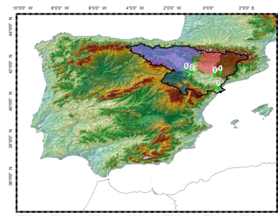
The study area we selected for this investigation is the Iberian Peninsula, which has three main climatic zones: Mediter-ranean, oceanic, and semiarid. The peninsula’s climate is pri-marily Mediterranean, except in its northern and southern parts, which are characterized mostly as oceanic and semi-arid, respectively. The topography varies from almost zero elevation to altitudes of 3500 m in the Pyrenees. For the hydrological analysis, we focused the study over the Ebro River basin and, specifically, on five subbasins of different spatial scale: (1) the Ebro River at Tortosa (84 230 km2); (2) the Ebro River at Zaragoza (40 434 km2); (3) the Cinca River at Fraga (9612 km2); (4) the Segre River at Lleida (11 369 km2); and (5) the Jalon River at Grisen (9694 km2) (Fig. 1). The datasets we used are described below.

2.1 Reference precipitation (SAFRAN)

Figure 1.Map of the Iberian Peninsula case study area.

this case were provided by the Spanish State Meteorolog-ical Agency (AEMET). The variables analyzed were pre-cipitation, temperature, relative humidity, wind speed, and cloudiness. In the case of precipitation, the first guess was deduced from the observations themselves instead of coming from a numerical model, like the other variables. The obser-vations were analyzed daily (as opposed to every 6 h for the other variables), but the resulting product had a time resolu-tion of 1 h. This was achieved by an interpolaresolu-tion method that used relative humidity to distribute precipitation throughout the day. Spatially, the outputs are presented on a regular grid with 5 km resolution. The dataset (Quintana-Seguí et al., 2016), which spans 35 years, covers mainland Spain and the Balearic Islands.

2.2 Satellite-based precipitation

We used three gauge-adjusted quasi-global satellite precip-itation products – CMORPH, PERSIANN, and 3B42 (V7) – in this study. CMORPH (Climate Prediction Center Mor-phing technique of the National Oceanic and Atmospheric Administration, or NOAA) is a global precipitation prod-uct based on passive microwave (PMW) satellite precipita-tion fields spatially propagated by moprecipita-tion vectors calculated from infrared (IR) data (Joyce et al., 2004). PERSIANN (Pre-cipitation Estimation from Remotely Sensed Information us-ing Artificial Neural Networks) is IR-based and uses a neu-tral network technique to connect IR observations to PMW rainfall estimates (Sorooshian et al., 2000). TMPA (Tropi-cal Rainfall Measuring Mission Multisatellite Precipitation Analysis), or 3B42 (V7), is a merged IR and passive mi-crowave precipitation product from NASA that is gauge-adjusted and available in both near-real time and post-real time (Huffman et al., 2010). Spatial and temporal resolutions

of the satellite precipitation products are 0.25◦and 3-hourly time intervals, respectively.

2.3 Atmospheric reanalysis

For meteorological forcing, we selected the WATCH1 (Wa-ter and Global Change FP7 project) Forcing Dataset ERA-Interim (hereafter WFDEI) (Weedon et al., 2014), a contem-porary state-of-the-art database. WFDEI, a dataset that fol-lows up on the European Union’s WATCH project (Hard-ing et al., 2011), is built on the ECMWF ERA-Interim re-analysis (Dee et al., 2011) with a geographical resolution of 0.5◦×0.5◦and a sequential frequency of 3 h for the time span 1979–2012, with particular bias corrections using gridded monitoring. Finally, we chose two atmospheric products (at-mospheric precipitation and air temperature) among WFDEI variables as predictors for the nonparametric statistical tech-nique.

2.4 Soil moisture

2.5 Terrain elevation

The Shuttle Radar Topography Mission (SRTM) dataset in-cluded in this study has, in recent years, been one of the most extensively used publicly accessible terrain elevation datasets. Available at ∼90 m spatial resolution, it was ob-tained using 1◦digital elevation model (DEM) tiles from the US Geological Survey and interpolated to the 0.25◦grid res-olution to match the resres-olution of precipitation and soil mois-ture products.

3 Methodology 3.1 Blending technique

In this study, we applied a nonparametric, tree-based re-gression model, quantile rere-gression forests (QRF) (Mein-shausen, 2006), to produce a rainfall ensemble with respect to the reference precipitation. The model input includes the three global satellite precipitation datasets (CMORPH, PER-SIANN, and 3B42-V7), the global reanalysis rainfall and air temperature datasets, and the satellite near-surface soil mois-ture and terrain elevation datasets, described in the previous section. The atmospheric products were interpolated in space using the nearest neighbor interpolation technique to match the resolution of precipitation satellite precipitation datasets. The spatial and temporal resolutions of the atmospheric prod-ucts are 0.25◦and 3-hourly time intervals, correspondingly. The high-resolution SAFRAN data were matched to the satellite precipitation datasets on a pixel-by-pixel basis by averaging all high-resolution pixels within a 0.25◦pixel. Fi-nally, all 3-hourly data were mapped to the grid resolution of 0.25◦chosen to be the final spatial resolution for the com-bined product.

QRF is derived from random forest regression (Mein-shausen, 2006), which is capable of handling data from large samples; it has desirable built-in features, such as variable se-lection, interaction detection, incorporation of missing data, and the ability to save the trained model for future predic-tion (Nateghi et al., 2014). QRF uses a bagged version (boot-strapped aggregating) of decision trees by randomly sam-pling from the bootstrapped sample, which reduces variance and helps to avoid overfitting that improves the stability and accuracy of the algorithm (Meinshausen, 2006). QRF pro-vides a nonparametric way to evaluate conditional quantiles for high-dimensional predictors of variables. The conditional distribution function ofY is defined by

ˆ

F (y|X=x)=P (Y ≤y|X=x)=E 1{Y≤y}|X=x, (1)

whereY refers to observations of the response variable,X

is a covariate or predictor variable, and E is the condi-tional mean,E(1{Y≤y}|X=x), which is approximated by the

weighted mean over the observation of 1{Y≤y}(Meinshausen,

2006). Then Eq. (1) can be expressed as

ˆ

F (y|X=x)= n

X

i=1

ωi(x)1{Yi≤y}, (2)

where weight vectorωi(x)=k−1Pik=1ωi(x, θt)using

ran-dom forest regression;kindicates the number of single trees (t=1, . . ., k); and each tree is built with an independent and identically distributed vectorθt (Meinshausen, 2006).

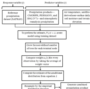
This nonparametric technique utilizes the weighted aver-age of all trees to compute the empirical distribution func-tion. It keeps not only the mean but also all observation val-ues in nodes and, building on this information, it calculates the conditional distribution. In this method, consistency of the empirical quantities is induced based on a large num-ber of instances in terminal nodes. The overall framework of the QRF scheme is shown in Fig. 2. Higher number of trees reduces the variance of the model. So, increasing the number of trees in the ensemble will not have any impact on the bias of the model. Furthermore, a higher variance reduc-tion can be achieved by decreasing the correlareduc-tion between trees in the ensemble. Therefore, QRF utilizes the optimal number “mtry” (size of the random subset of predictors) for split point selection at each node. This approach introduces randomness in the ensemble to reduce the correlation be-tween trees, which helps to avoid overfitting (Meinshausen, 2006). In this study we used the default value (k=1000) (Meinshausen, 2006) throughout all simulations to create the empirical distribution at each grid cell and used the cross-validation experiments (see next section) to demonstrate sta-bility of the method.

Specifically, we initialized a random forest of 1000 trees for each terminal node of each of the classified dataset and calculated the 95 % prediction intervals at each grid cell. QRF utilizes the same weights to calculate the empirical dis-tribution function and a weighted average of all trees for the predicted expected response values to calculate the empirical distribution. To conduct the hydrological simulations in this study, we resampled from the empirical distribution function 20 times per grid cell to obtain “reference”-like rainfall en-semble members.

calibra-Figure 2.A schematic representation of the quantile regression forests (QRF) framework used.

tion of the technique. In general, prominent “mtry” is ob-tained by this method by extending the sample size and there-fore preventing overfitting. Applying this validation method, the model exhibits great skill on both the training dataset and the unseen test data. Similarly, to strengthen the valida-tion results, we also performed a test using leave-one-year-out cross-validation. Namely, for each year of the database hold out for validation, we calibrated on the rest of the years (10 years) and repeated the experiment for all 11 years of the study period. The model validation results based on leave-one-pixel-out and leave-one-year-out are described in Sect. 4.2.

3.2 Hydrological modeling

To perform the streamflow simulations, we used the SASER (SAfran-Surfex-Eaudyssée-Rapid) hydrological modeling suite. SASER is a physically based and distributed hydro-logical model for Spain based on SURFEX (Surface Ex-ternalisée), a land surface modeling platform developed by Météo-France (Masson et al., 2013) that integrates several schemes for different kinds of surfaces (natural, urban, lakes, and so on). The scheme for natural surfaces, ISBA (Noilhan and Planton, 1989; Noilhan and Mahfouf, 1996), has differ-ent versions, with differing degrees of complexity. Within SASER we used the explicit multilayer version (Boone,

2000; Decharme et al., 2011) with prescribed vegetation. The physiography was provided by the ECOCLIMAP dataset (Champeaux et al., 2005).

Since SURFEX has no river routing scheme, we chose the RAPID river routing scheme (David et al., 2011a, b) within the Eau-dyssée framework (http://www.geosciences.mines-paristech.fr/fr/equipes/ systemes-hydrologiques-et-reservoirs/projets/eau-dyssee). Eau-dyssée transfers SURFEX runoff (surface and sub-surface or drainage) from the SURFEX grid cells to the river cells using its own isochrony algorithm. Then, RAPID uses a matrix-based version of the Muskingum method to calculate flow and volume of water for each reach of a river network. The current application of SASER uses HYDROSHEDS (Lehner et al., 2008) to describe the river network. As the current setup cannot simulate dams, canals, or irrigation, the resulting river flows are estimations of the natural system (that is, the system without direct human intervention in the form of irrigation or hydraulic infrastructure, such as dams or canals).

applications of SURFEX, which are not calibrated either. The downside is that the model might not perform optimally. In the future, we plan to improve the options used in the land surface model to adapt its structure better to the necessary physical processes that take place in the basin, while limiting the need for parameter calibration. For the purpose of this study, which involved the relative comparison of multiple rainfall forcing-based simulations, the current model setup was considered adequate.

3.3 Metrics of model performance evaluation

We based quantification of the systematic and random error of model-generated ensemble on different error metrics. We evaluated the random error component based on the normal-ized centered root mean square error (NCRMSE), which is defined as NCRMSE= r 1 n Pn

i=1 h

ˆ

yi−yi−1 n

Pn

i=1 yiˆ −yi i2

1

n

Pn i=1yi

. (3)

Note thatyi is reference rainfall,yiˆ is estimated rainfall for times i from the blended technique, andn is the total number of data points used in the calculations. An NCRMSE value of 0 indicates no random error, while 1 indicates that the random error is equal to 100 % of the mean reference rainfall.

To measure the systematic error, we used the bias ratio (BR) metric, which indicates the mean of the ratio of esti-mated rainfall to reference rainfall and is defined as

BR=1 n

n

X

i=1 _yiˆ

yi

. (4)

For an unbiased model, the BR would be 1.

To assess the ability of the QRF-generated ensemble to encapsulate the reference rainfall, we used the exceedance probability (EP) metric, which indicates the probability that the reference value will exceed the prediction interval: EP=1−1

n n

X

i=1 1n

Qloweri<yi<Qupper_i

o. (5) Here,QlowerandQupperdenote lower and upper boundaries of prediction interval, respectively. The EP would be 0 for an ideal model; that means a perfect encapsulation of the refer-ence within the prediction interval.

To evaluate the accuracy of the QRF-generated ensemble, we used the uncertainty ratio (UR), which measures uncer-tainty from the prediction interval (Qlower,Qupper), as used in Eq. (3):

UR= Pn

i=1 Qupper−Qlower Pn

i=1yi

. (6)

To achieve accurate and successful prediction, compara-tively small prediction intervals are expected. A UR value of

1 means the best estimate of the actual uncertainty which in-dicates the maximum possible uncertainty of the prediction interval. The UR quantifies the prediction interval width rel-ative to the magnitude of observations. A UR value close to 1 indicates confidence intervals being in the order of magni-tude of the predicted values.

For the evaluation of the accuracy of the ensemble, we also calculated the rank histogram, which is computed by count-ing the rank of observations and comparcount-ing this with values from a compiled ensemble, in ascending order. The rank of the actual value is denoted byrj(r1, r2, . . ., rm+1)andrj is

expressed as follows:

rj = ˆP{ ˆyi,j−1< yi<yi,jˆ }. (7)

A flat rank histogram diagram means precise prediction of error distribution (Hamil, 2001; Hamil and Colucci, 1997). A U-shaped rank histogram (convex) represents conditional biases, and a concave shape means an over-spread. Skewing to the right denotes negative bias and vice versa.

The Nash–Sutcliffe efficiency (NSE) is widely used in hy-drology to assess model performance (Nash and Sutcliffe, 1970) and is defined as

NSE=1− Pn

i=1 yˆi−yi

2

Pn

i=1(yi−y)2

. (8)

The NSE bounds from negative infinity to positive 1, where positive 1 means ideal consistency. A negative value of NSE denotes the performance of the estimator being worse than the mean of reference.

4 Results and discussion 4.1 Sensitivity analysis

controlled surface soil moisture data with a global coverage and 0.25◦ _{spatial resolution while the available vegetation}

indices are provided at much coarser (multi-day) temporal scales. Also the precipitation products, despite using similar observations to some extent, exhibit different error character-istics and could provide complementary information. There-fore, dynamic (temperature and soil moisture) and static (el-evation) land surface variables were used as input along with the multiple global precipitation sources (CMORPH, PER-SIANN, and 3B42 (V7); and atmospheric reanalysis precipi-tation).

After choosing these predictor variables, for any nonpara-metric statistical technique, it is essential to know the sen-sitivity of the result to the different input predictor vari-ables and to quantify the impact of change from one variable to another. The variable importance methodology (Breiman, 2001) is a measure of sensitivity in that case, which helps to recognize crucial input variables that demonstrate the rel-ative contribution of each variable. The importance of the predictor variables depends on the magnitude of the per-centage increase in mean square error (% IncMSE) of the model (Breiman, 2001). Higher values of % IncMSE indi-cate higher importance of the predictor variables. Briefly, the mean squared error (MSE) computed from the original model (i.e., considering all variables) is compared against MSE from a new model that holds all variables the same as the original model except one, the one of which we want to determine its relative importance.

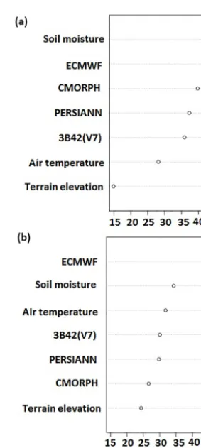
Results from the variable importance test show that all variables used in this technique contribute valuable infor-mation in the modeling process. Results from the variable importance test for two groups included in our methodol-ogy (for warm and cold periods, high elevation and rainfall greater than zero for all products) are presented in Fig. 3, which shows the variable importance of the seven predictor variables. According to these results all variables are impor-tant but the level of significance varies considerably among the different variables. Soil moisture, reanalysis, and the three satellite precipitation datasets were ranked as the most important predictor variables (Fig. 3), showing their strong impact in model prediction. Similar results (not shown) were obtained from examination of the other scenarios (e.g., for low elevation cases). From the variable importance test, it is argued that all variables selected have a significant impact on the model prediction, justifying our choice for including them.

4.2 Evaluation of the blending technique

We first evaluated the method by applying a leave-one-pixel-out cross validation, where each pixel was treated as an inde-pendent dataset and was predicted based on QRF parameters determined based on the remaining pixels in the database. The time series of 20 ensemble members’ cumulative rain-fall simulated by QRF for high and low elevations in warm

Figure 3.Variable importance plot, where % IncMSE is the percent-age increase in mean square error.(a)Warm period–high elevation. (b)Cold period–high elevation.

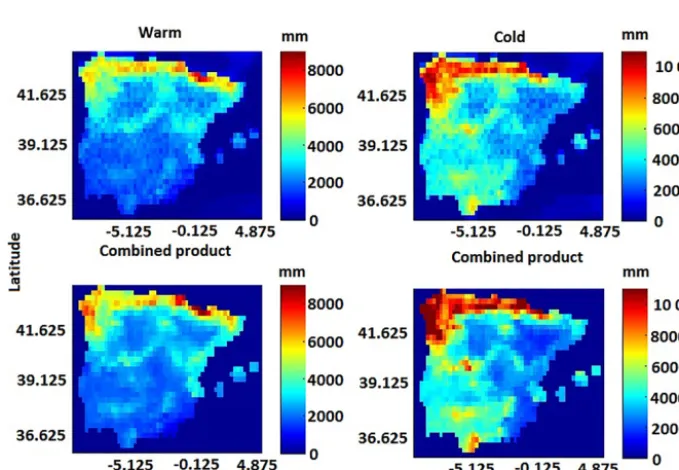
and cold seasons are shown in Fig. 4. The ensemble enve-lope encapsulates the actual rainfall time series, with better convergence of QRF ensemble members for the warm season but with overall satisfying results for the cold season as well. As is shown, the model was capable of generating stochastic realizations that successfully encapsulated the reference pre-cipitation dynamics. Apart from the ensemble performance, one can note from the results in Fig. 4 the variability in the performance of different precipitation products and their in-consistencies relative to the reference precipitation. For ex-ample, PERSIANN overestimated high elevation in the warm season, while CMORPH, 3B42 (V7), and atmospheric re-analysis precipitation underestimated it. Overall, CMORPH underestimated the most for both seasons, which indicated poor performance of the QRF ensemble.

Figure 4.Time series of cumulative rainfall of CMORPH, PERSIANN, 3B42 (V7), reanalysis rainfall, and QRF ensemble (blue envelope) for warm and cold seasons.

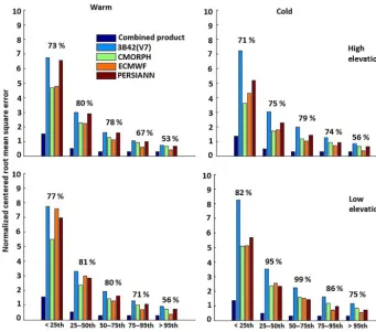
Figure 6.Normalized centered root mean square error for warm and cold seasons. The relative error reductions for the combined product (relative to other products) are shown above the bars.

the Iberian Peninsula than in the warm season. These pat-terns were consistent with those presented in the reference dataset.

We calculated NCRMSE for the various precipitation products (Fig. 6) for five reference precipitation categories, with values in the percentile ranges of<25th, 25th–50th, 50th–75th, 75th–95th, and>95th. The results showed the QRF-based combined product could reduce the random er-ror for all rainfall rate categories in both seasons. It is also shown that the random error reduced consistently in all prod-ucts as the rainfall rate increased.

To quantify the performance of the combined product in contrast to the individual precipitation datasets, we calcu-lated the relative reduction of the NCRMSE for the differ-ent precipitation ranges; Fig. 6 presdiffer-ents these performance metric statistics. The relative reduction of the values was defined as the difference between the average of the dif-ferent datasets and the combined product over the average NCRMSE of the datasets. We noted that relative NCRMSE reduction was greater during the cold season, particularly in regions of low elevation (75 to 99 %). During the warm sea-son, the relative reduction varied between 53 and 81 % for both high and low elevations. Overall, results from all met-rics examined showed that the random error of the combined

product was significantly lower than those of the individual global precipitation datasets used in the technique.

Figure 7.Bias ratio for warm and cold seasons.

the systematic error at high elevations noticeably. For the higher rain rate category (>95th percentile), the BR value in the warm season ranged between 0.5 and 0.6, which was close to estimations for the cold season over the study area. The relative reduction was high for the combined product, varying from 17 to 76 % for both seasons. Overall, the com-bined product exhibited BR values closer to 1 than the indi-vidual precipitation datasets did, demonstrating superior per-formance.

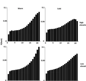
Results for exceedance probability (EP) values (Fig. 8), which are used to assess the ability of the QRF-generated ensemble to encapsulate the reference data, suggest that ref-erence precipitation is captured well within the ensemble en-velope. Specifically, considerably reduced exceedance prob-ability values (<0.26) were reported for rain rates below the 95th percentile threshold for both seasons. A season-based comparison revealed that cold-season EP values were smaller than the corresponding values for the warm season across all rain rate thresholds. Even for the high rain rates (>95th per-centile), EP values were found to be acceptable (∼0.5).

Analysis of UR showed the QRF ensemble envelope was associated with slightly wider prediction intervals in the warm season than in the cold season, indicating varying

de-grees of uncertainty throughout the year (Fig. 8). A UR closer to 1 was exhibited for higher rain rates, demonstrating that the ensemble envelope represented the uncertainty for the moderate to high rain rates well, while the variability of the ensemble envelope for rain rates below the 50th percentile threshold overestimated the product uncertainty.

Finally, to evaluate the accuracy of the QRF ensemble, we calculated the rank histogram for the cold and warm seasons. Figure 9 shows the rank histogram of reference values in the posterior sample of QRF ensemble prediction for both seasons. QRF produced a nearly uniformly distributed rank histogram for low to moderate rain rates, which means the rank test was more promising for QRF ensemble predictions for these rain rates. However, the rank histogram exhibited larger values on the right-hand side, indicating underestima-tion of high rain rates in the ensemble predicunderestima-tion, which is potentially attributed to the inclusion of the entire spectrum of values in the training dataset (i.e., large sample of zeroes and low values) that although allow for reproducing certain important features of precipitation (e.g., intermittency), im-pact the simulation of high rainfall regime.

Figure 8.Exceedance probability and uncertainty ratio for warm and cold seasons.

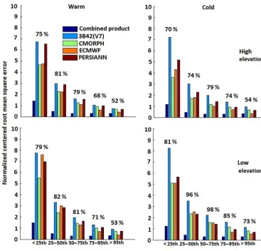
Figure 10.Normalized centered root mean square error for warm and cold season. The relative error reductions for the combined product (relative to other products) are shown above the bars.

independent dataset and the model was trained on the re-maining years of the study period. Results for NCRMSE are shown in Fig. 10, which are consistent with the leave-one-pixel-out cross-validation analysis in terms of the reduction of the random error for both seasons (warm and cold) and precipitation percentile ranges. The random error decreases with increasing scale, and for all cases, results from the com-bined product are associated with an error reduction (relative to other products) on the order of 52–98 %. Overall, results indicate that the random error of the combined product was significantly lower than those of the individual precipitation products used in this study.

The performance of the estimates for the model was also evaluated in terms of systematic error, as shown in Fig. 11. Results show that the magnitude of systematic error for the combined product is substantially lower than for the individ-ual precipitation products. Overall, BR values are closer to 1 for moderate to high rain rates in both seasons for the com-bined product, which indicates that QRF is able to reduce the systematic error in moderate to high rain rates.

In summary, both validation approaches demonstrated that the QRF model is able to reduce the systematic and random error of precipitation estimates exhibited by individual pre-cipitation products significantly, which indicates that QRF was appropriately trained and does not exhibit limitations due to overfitting. To conduct the hydrological simulations in this study, the validation of the results based on the leave-one-pixel-out method is provided in Sect. 4.3.

Figure 11.Bias ratio for warm and cold seasons.

used here to assess the performance of basin-scale precipita-tion forcing data and corresponding generated streamflows.

Since SASER does not simulate dams or canals or irriga-tion, the simulated streamflow reflects how the flow would be if the water resources of the basin were not managed (that is, naturalized streamflow). The Ebro basin is heavily managed, with hundreds of dams and an important canal network. This raised the problem that model flows could not be compared to the observed flows on those subbasins that are influenced by water management, which is most of them. The Spanish Ministry of Agriculture, Fisheries, Food, and the Environ-ment (MAPAMA) had, however, produced monthly natural-ized river flows using the SIMPA rain-runoff model (Ruiz et al., 1998; Álvarez et al., 2004). These are the reference val-ues used by the managers, and they currently offer the only means of reference for validating SASER results.

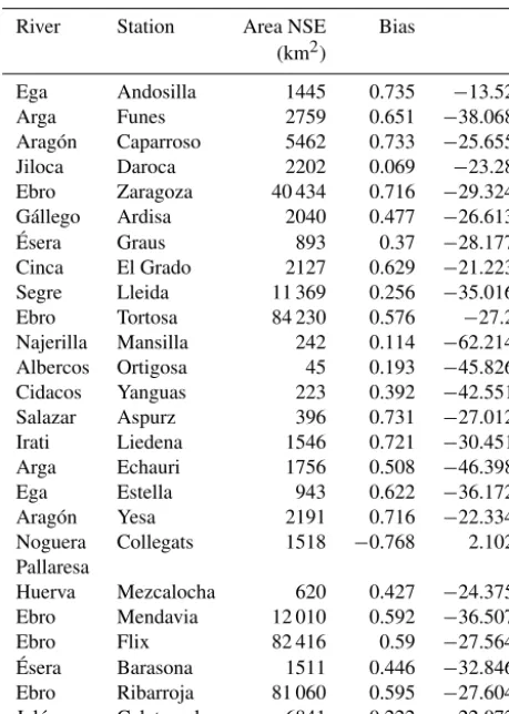
Table 1 compares the bias and NSE of SASER to those of SIMPA. In terms of monthly accumulation of precipita-tion, the precipitation data used by SIMPA were similar to SAFRAN’s; thus, the difference may have resided in evap-otranspiration, which is calculated differently in both

mod-els, in terms of both formulation and land-use maps. In terms of NSE, the scores are acceptable at the outlet (between 0.4 and 0.6) and better at most Pyrenean basins (between 0.4 and 0.8), with some exceptions.

Table 1.The bias and NSE of high-resolution SAFRAN-SURFEX simulation.

River Station Area NSE Bias

(km2)

Ega Andosilla 1445 0.735 −13.52

Arga Funes 2759 0.651 −38.068

Aragón Caparroso 5462 0.733 −25.655

Jiloca Daroca 2202 0.069 −23.28

Ebro Zaragoza 40 434 0.716 −29.324

Gállego Ardisa 2040 0.477 −26.613

Ésera Graus 893 0.37 −28.177

Cinca El Grado 2127 0.629 −21.223

Segre Lleida 11 369 0.256 −35.016

Ebro Tortosa 84 230 0.576 −27.2

Najerilla Mansilla 242 0.114 −62.214

Albercos Ortigosa 45 0.193 −45.826

Cidacos Yanguas 223 0.392 −42.551

Salazar Aspurz 396 0.731 −27.012

Irati Liedena 1546 0.721 −30.451

Arga Echauri 1756 0.508 −46.398

Ega Estella 943 0.622 −36.172

Aragón Yesa 2191 0.716 −22.334

Noguera Collegats 1518 −0.768 2.102

Pallaresa

Huerva Mezcalocha 620 0.427 −24.375

Ebro Mendavia 12 010 0.592 −36.507

Ebro Flix 82 416 0.59 −27.564

Ésera Barasona 1511 0.446 −32.846

Ebro Ribarroja 81 060 0.595 −27.604

Jalón Calatayud 6841 0.222 −22.072

To provide an overview of the differences in error mag-nitude between forcing and response variables, we present our analysis of error metrics for simulated streamflow along with corresponding error metrics in basin-average precipita-tion. Results for NCRMSE are shown in Fig. 12, which notes that for the two larger basins, Ebro at Tortosa (84 230 km2) and Ebro at Zaragoza (40 434 km2), the NCRMSE (0.1–0.3) of the combined product was significantly lower than those of the other subbasins for all intervals of streamflow values; this was related to the significant smoothing effect on random error associated with larger basin scales.

Consistent with streamflow, these two basins also exhib-ited considerably lower NCRMSE values (0.2–0.5) for the combined product in terms of basin-average precipitation. The random component of error was generally slightly higher for low precipitation rates than for the moderate and higher rates for the five subbasins. Similar findings in NCRMSE values for the low streamflow rates were observed. For the basin-average precipitation, the relative NCRMSE reduc-tion was high for the combined product, ranging from 84 to 88 % (below the 25th percentile group). A product-wise comparison showed the combined product had more sig-nificant error-dampening effects than reanalysis and

satel-lite precipitation products in streamflow simulation for all the subbasins. Specifically, the combined product (above the 50th percentile) was characterized by a noticeably rel-ative error reduction (44 to 78 %) for streamflow. Moreover, we also observed that relative error reduction for the com-bined product decreased remarkably (56 to 88 %) for low streamflow. These results indicated random error was re-duced through the rainfall–streamflow transformation in all subbasins. Overall, results show combining information from reanalysis and satellite precipitation datasets could decrease random error in streamflow simulations.

The bias ratio (BR) for basin-average precipitation ranges from overestimation to underestimation as a function of precipitation magnitude, with precipitation rates above the 50th percentile strongly underestimated (BR in the range of 0.07–0.25) (Fig. 13). The magnitude of BR for precipita-tion indicated lower systematic errors in estimates of low to high basin-average precipitation for all subbasins. The corre-sponding BR values for the simulated streamflows provided a general appreciation of how the magnitude of systematic error in basin-average precipitation translates to systematic error in streamflow simulations. While a one-to-one corre-spondence between rainfall and streamflow classes was not possible (note that an event from the highest rainfall class might have resulted in moderate flow values depending on antecedent conditions and so on), we could, however, com-pare the overall range of BR values between basin-average precipitation and streamflow. As Fig. 13 indicates for the combined product, BR values were closer to 1 for the dif-ferent streamflow classes, indicating that streamflow was rel-atively stable. For the two larger basins, Ebro at Tortosa and Ebro at Zaragoza, the combined product underestimated ac-tual values slightly. Overall, the relative systematic error duction for streamflow ranged from 20 to 99 %. These re-sults highlight the usefulness of optimally combining satel-lite and reanalysis precipitation datasets. Overall, after reduc-ing systematic error, the QRF-generated ensemble correc-tions brought rainfall products closer to the reference rainfall and simulated runoff.

5 Conclusions

Figure 12.Normalized centered root mean square error for basin-average rainfall and streamflow. The relative error reductions for the combined product (relative to other products) are shown above the bars.

evaluated against the SAFRAN-based simulations for a range of basin scales of the Ebro River basin.

Results from the analysis carried out demonstrate clearly that the proposed blending technique has the potential to gen-erate a realistic precipitation ensemble that is statistically consistent with the reference precipitation and is associated with considerably reduced errors. In terms of seasonality ef-fects, the random error significantly decreased for the com-bined product with increasing rainfall magnitude, and this reduction was greater during the cold season. The systematic error of the combined product varied from over- to underes-timation as rain rate increased during both seasons. In terms of elevation, among all individual products, the magnitude of systematic error for the combined product was noticeably de-creased for the higher elevations, which is a strong indication for using the proposed scheme in retrieving global precipita-tion in high-elevaprecipita-tion regions. Overall, the reducprecipita-tion of the combined product (relative to other products) for the

system-atic and random error ranged between 17 and 76 and 53 and 99 %, respectively.

Evaluation of the impact on streamflow simulations showed that the magnitude of systematic and random error for simulations corresponding to the combined product was significantly lower than for the individual precipitation prod-ucts. In addition, for the combined product, the large-scale basins exhibited considerably lower systematic and random error values than the small-size basins, which shows the de-pendency on basin scale. Specifically, the relative reduction for the combined product in systematic and random error ranged between 20 and 99 and 44 and 88 %, respectively, which highlights the potential of the proposed technique in advancing hydrologic simulations.

Figure 13.Bias ratio of precipitation and streamflow.

have important applications in studies dealing with water re-sources reanalysis and quantification of uncertainty in hydro-logic simulations. Future work will include evaluation of the proposed framework in different hydroclimatic regions, also considering the sensitivity of its performance to availability (e.g., record length and spatial coverage) of in situ reference precipitation.

Data availability. Several datasets were used for this pa-per. The SAFRAN dataset for Spain was obtained from the MISTRALS HyMeX database (https://doi.org/10.14768/ MISTRALS-HYMEX.1388). The other datasets are also available online: CMORPH (ftp://ftp.cpc.ncep.noaa.gov/ precip/CMORPH_V1.0/RAW/0.25deg-3HLY/), PERSIANN (http://fire.eng.uci.edu/PERSIANN/data/3hrly_adj_cact_tars/), 3B42 (V7) (https://mirador.gsfc.nasa.gov), atmospheric reanalysis dataset (https://wci.earth2observe.eu/portal/), satellite-derived near-surface daily soil moisture data (http://www.esa-soilmoisture-cci.org/node/145/), terrain elevation data (http://srtm.csi.cgiar.org/SELECTION/inputCoord.asp),

and the combined product (https://sites.google.com/uconn.edu/ ehsanbhuiyan/research).

Competing interests. The authors declare that they have no conflict of interest.

Acknowledgements. This research was supported by the FP7 project eartH2Observe (grant agreement no. 603608).

Edited by: Hannah Cloke

References

Adler, R. F., Kidd, C., Petty, G., Morissey, M., and Goodman, H. M.: Intercomparison of global precipitation products: the third pre-cipitation intercomparison project (PIP–3), B. Am. Meteorol. Soc., 82, 1377–1396, 2001.

AghaKouchak, A., Nasrollahi, N., and Habib, E.: Accounting for uncertainties of the TRMM Satellite Estimates, Remote Sens., 1, 606–619, 2009.

Álvarez, J., Sánchez, A., and Quintas, L.: SIMPA, a GRASS based tool for hydrological studies, in: Proceedings of the FOSS/GRASS Users Conference, Bangkok, Thailand, 2004. Bhuiyan, M. A. E., Anagnostou, E. N, and Kirstetter, P. E.:

A nonparametric statistical technique for modeling overland TMI (2A12) rainfall retrieval error, IEEE Geosci. Remote S., 14, 1898–1902, 2017.

Bitew, M. M. and Gebremichael, M.: Evaluation of satellite rain-fall products through hydrologic simulation in a fully dis-tributed hydrologic model, Water Resour. Res., 47, W06526, https://doi.org/10.1029/2010WR009917, 2011.

Boone, A.: Modélisation des processus hydrologiques dans le schéma de surface ISBA: Inclusion d’un réservoir hydrologique, du gel et modélisation de la neige, Université Paul Sabatier (Toulouse III), Toulouse, available at: http://www.cnrm.meteo.fr/ IMG/pdf/boone_thesis_2000.pdf, 2000.

Breiman, L.: Random forests, Mach. Learn., 45, 5–32, 2001. Brown, J. D. and Seo, D. J.: A nonparametric postprocessor for

bias correction of hydrometeorological and hydrologic ensemble forecasts, J. Hydrometeorol., 11, 642–665, 2010.

Champeaux, J. L., Masson, V., and Chauvin, F.: ECOCLIMAP: a global database of land surface parameters at 1 km resolution, Meteorol. Appl., 12, 29–32, 2005.

Chipman, H. A., George, E. I., and McCulloch, R. E.: Bart: Bayesian additive regression trees, Ann. Appl. Stat., 4, 266–298, 2010.

Ciach, G. J., Krajewski, W. F., and Villarini, G.: Product-error-driven uncertainty model for probabilistic quantitative precipita-tion estimaprecipita-tion with NEXRAD data, J. Hydrometeorol., 8, 1325– 1347, https://doi.org/10.1175/2007JHM814.1, 2007.

Croley, T. E.: Weighted-climate parametric hydrologic forecasting, J. Hydrol. Eng., 8, 8171–8180, 2003.

David, C. H., Maidment, D. R., Niu, G. Y., Yang, Z. L., Habets, F., and Eijkhout, V.: River network routing on the NHDPlus dataset, J. Hydrometeorol., 12, 913–934, 2011a.

David, C. H., Habets, F., Maidment, D. R., and Yang, Z. L.: RAPID applied to the SIM-France model, Hydrol. Process., 25, 3412– 3425, 2011b.

De Jeu, R. A.: Retrieval of land surface parameters using passive microwave remote sensing, PhD Dissertation, VU Amsterdam, the Netherlands, 120 pp., 2003.

Decharme, B., Boone, A., Delire, C., and Noilhan, J.: Lo-cal evaluation of the interaction between soil biosphere atmosphere soil multilayer diffusion scheme using four pedotransfer functions, J. Geophys. Res.-Atmos., 116, https://doi.org/10.1029/2011JD016002, 2011.

Dee, D. P., Uppala, S. M., Simmons, A. J., Berrisford, P., Poli, P., Kobayashi, S., Andrae, U., Balmaseda, M. A., Balsamo, G., Bauer, P., and Bechtold, P.: The ERA-Interim reanalysis: con-figuration and performance of the data assimilation system, Q. J. Roy. Meteor. Soc., 137, 553–597, 2011.

Derin, Y., Anagnostou, E., Berne, A., Borga, M., Boudevillain, B., Buytaert, W., Chang, C. H., Delrieu, G., Hong, Y., Hsu, Y. C., and Lavado-Casimiro, W.: Multiregional satellite precipitation products evaluation over complex terrain, J. Hydrometeorol., 17, 1817–1836, https://doi.org/10.1175/JHM-D-15-0197.1, 2016. Durand, Y., Brun, E., Merindol, L., Guyomarc’h, G., Lesaffre, B.,

and Martin, E.: A meteorological estimation of relevant parame-ters for snow models, Ann. Glaciol., 18, 65–71, 1993.

Francke, T., López-Tarazón, J. A., Vericat, D., Bronstert, A., and Batalla, R. J.: Flood-based analysis of high-magnitude sedi-ment transport using a non-parametric method, Earth Surf. Proc. Land., 33, 2064–2077, 2008.

Gebremichael, M., Liao, G. Y., and Yan, J.: Nonpara-metric error model for a high resolution satellite rainfall product, Water Resour. Res., 47, W07504, https://doi.org/10.1029/2010WR009667, 2011.

Gottschalck, J., Meng, J., Rodell, M., and Houser, P.: Anal-ysis of multiple precipitation products and preliminary as-sessment of their impact on global land data assimilation system land surface states, J. Hydrometeorol., 6, 573–598, https://doi.org/10.1175/JHM437.1, 2005.

Guikema, S. D., Quiring, S. M., and Han, S. R.: Prestorm estimation of hurricane damage to electric power distribution systems, Risk Anal., 30, 1744–1752, 2010.

Hamill, T. M.: Interpretation of rank histograms for verifying en-semble forecasts, Mon. Weather Rev., 129, 550–560, 2001. Hamill, T. M. and Colucci, S. J.: Verification of Eta–RSM

short-range ensemble forecasts, Mon. Weather Rev., 125, 1312–1327, 1997.

Harding, R., Best, M., Blyth, E., Hagemann, S., Kabat, P., Tal-laksen, L. M., Warnaars, T., Wiberg, D., Weedon, G. P., La-nen, H. V., and Ludwig, F.: WATCH: current knowledge of the terrestrial global water cycle, J. Hydrometeorol., 12, 1149–1156, 2011.

He, J., Wanik, D., Hartman, B., Anagnostou, E., Astitha, M., and Frediani, M. E. B.: Nonparametric tree-based predictive model-ing of storm damage to power distribution network, Risk Anal., 37, 441–458, https://doi.org/10.1111/risa.12652, 2017.

Hossain, F. and Anagnostou, E. N.: Assessment of current passive-microwave- and infrared-based satellite rainfall remote sens-ing for flood prediction, J. Geophys. Res., 109, D07102, https://doi.org/10.1029/2003JD003986, 2004.

Hossain, F. and Anagnostou, E. N.: Assessment of a multidimen-sional satellite rainfall error model for ensemble generation of satellite rainfall data, IEEE Trans. Geosci. Remote Sens. Lett., 3, 419–423, 2006.

Hou, A. Y., Kakar, R. K., Neeck, S., Azarbarzin, A. A., Kum-merow, C. D., Kojima, M., Oki, R., Nakamura, K., and Iguchi, T.: The global precipitation measurement mission, B. Am. Mete-orol. Soc., 95, 701–722, https://doi.org/10.1175/BAMS-D-13-00164.1, 2014.

Huffman, G. J., Bolvin, D. T., Nelkin, E. J., Wolff, D. B., Adler, R. F., Gu, G., Hong, Y., Bowman, K. P., and Stocker, E. F.: The TRMM Multisatellite Precipitation Analy-sis (TMPA): quasi-global, multiyear, combined-sensor precip-itation estimates at fine scales, J. Hydrometeorol., 8, 38–55, https://doi.org/10.1175/JHM560.1, 2007.

Satel-lite rainfall applications for surface hydrology, edited by: Ge-bremichael, M. and Hossain, F., Springer, Dordrecht, 3–22, 2010. Joyce, R. J., Janowiak, J. E., Arkin, P. A., and Xie, P.: CMORPH: a method that produces global precipitation estimates from pas-sive microwave and infrared data at high spatial and temporal resolution, J. Hydrometeorol., 5, 487–503, 2004.

Juban, J., Fugon, L., and Kariniotakis, G.: Probabilistic short-term wind power forecasting based on kernel density estimators, in: European Wind Energy Conference and exhibition, EWEC 2007, 7–10 May 2017, Milan, Italy, 2007.

Lakhankar, T., Ghedira, H., Temimi, M., Sengupta, M., Khanbil-vardi, R., and Blake, R.: Non-parametric methods for soil mois-ture retrieval from satellite remote sensing data, Remote Sens.-Basel, 1, 3–21, https://doi.org/10.3390/rs1010003, 2009. Lehner, B., Verdin, K., and Jarvis, A.: New global hydrography

de-rived from spaceborne elevation data, Eos, 89, 93–94, 2008. Li, L., Hong, Y., Wang, J., Adler, R. F., Policelli, F. S.,

Habib, S., Irwn, D., Korme, T., and Okello, L.: Evalua-tion of the real-time TRMM-based multi-satellite precipita-tion analysis for an operaprecipita-tional flood predicprecipita-tion system in Nzoia basin, Lake Victoria, Africa, Nat. Hazards, 50, 109–123, https://doi.org/10.1007/s11069-008-9324-5, 2009.

Liu, Y. Y., Parinussa, R. M., Dorigo, W. A., De Jeu, R. A. M., Wagner, W., van Dijk, A. I. J. M., McCabe, M. F., and Evans, J. P.: Developing an improved soil moisture dataset by blending passive and active microwave satellite-based retrievals, Hydrol. Earth Syst. Sci., 15, 425–436, https://doi.org/10.5194/hess-15-425-2011, 2011.

Liu, Y. Y., Dorigo, W. A., Parinussa, R. M., de Jeu, R. A., Wag-ner, W., McCabe, M. F., Evans, J. P., and Van Dijk, A. I. J. M.: Trend-preserving blending of passive and active microwave soil moisture retrievals, Remote Sens. Environ., 123, 280–297, 2012. Maggioni, V., Sapiano, M. R., Adler, R. F., Tian, Y., and Huff-man, G. J.: An error model for uncertainty quantification in high-time-resolution precipitation products, J. Hydrometeorol., 15, 1274–1292, https://doi.org/10.1175/JHM-D-13-0112.1, 2014. Maggioni, V., Massari, C., Brocca, L., and Ciabatta, L.: Merging

bottom-up and top-down precipitation products using a stochas-tic error model, J. Geophys. Res., 19, 12383, 2017.

Masson, V., Le Moigne, P., Martin, E., Faroux, S., Alias, A., Alkama, R., Belamari, S., Barbu, A., Boone, A., Bouyssel, F., Brousseau, P., Brun, E., Calvet, J.-C., Carrer, D., Decharme, B., Delire, C., Donier, S., Essaouini, K., Gibelin, A.-L., Giordani, H., Habets, F., Jidane, M., Kerdraon, G., Kourzeneva, E., Lafaysse, M., Lafont, S., Lebeaupin Brossier, C., Lemonsu, A., Mahfouf, J.-F., Marguinaud, P., Mokhtari, M., Morin, S., Pigeon, G., Sal-gado, R., Seity, Y., Taillefer, F., Tanguy, G., Tulet, P., Vincendon, B., Vionnet, V., and Voldoire, A.: The SURFEXv7.2 land and ocean surface platform for coupled or offline simulation of earth surface variables and fluxes, Geosci. Model Dev., 6, 929–960, https://doi.org/10.5194/gmd-6-929-2013, 2013.

Mei, Y., Anagnostou, E. N., Nikolopoulos, E. I., and Borga, M.: Error analysis of satellite rainfall products in mountainous basins, J. Hydrometeorol., 15, 1778–1793, https://doi.org/10.1175/JHM-D-13-0194.1, 2014.

Mei, Y., Nikolopoulos, E. I., Anagnostou, E. N., and Borga, M.: Evaluating satellite precipitation error propagation in runoff sim-ulations of mountainous basins, J. Hydrometeorol., 17, 1407– 1423, https://doi.org/10.1175/JHM-D-15-0081.1, 2016.

Meinshausen, N.: Quantile regression forests, J. Mach. Learn. Res., 7, 983–999, 2006.

Mo, K. C., Chen, L. C., Shukla, S., Bohn, T. J., and Letten-maier, D. P.: Uncertainties in North American land data assim-ilation systems over the contiguous United States, J. Hydromete-orol., 13, 996–1009, https://doi.org/10.1175/JHM-D-11-0132.1, 2012.

Mujumdar, P. P. and Ghosh, S.: Climate change impact on hydrol-ogy and water resources, J. Hydraul. Eng., 14, 1–17, 2008. Nash, J. E. and Sutcliffe, J. V.: River flow forecasting through

con-ceptual models part I – a discussion of principles, J. Hydrol., 10, 282–290, 1970.

Nateghi, R., Guikema, S. D., and Quiring, S. M.: Forecasting hurricane-induced power outage durations, Nat. Hazards, 74, 1795–1811, 2014.

Nikolopoulos, E. I., Anagnostou, E. N., and Borga, M.: Using high-resolution satellite rainfall products to simulate a major flash flood event in Northern Italy, J. Hydrometeorol., 14, 171–185, https://doi.org/10.1175/JHM-D-12-09.1, 2013.

Noilhan, J. and Mahfouf, J. F.: The ISBA land surface parameteri-sation scheme, Global Planet. Change, 13, 145–159, 1996. Noilhan, J. and Planton, S.: A simple parameterization of land

sur-face processes for meteorological models, Mon. Weather Rev., 117, 536–549, 1989.

Owe, M., de Jeu, R., and Holmes, T.: Multisensor historical clima-tology of satellite-derived global land surface moisture, J. Geo-phys. Res., 113, F01002, https://doi.org/10.1029/2007JF000769, 2008.

Peña-Arancibia, J. L., van Dijk, A. I., Renzullo, L. J., and Mulli-gan, M.: Evaluation of precipitation estimation accuracy in re-analyses, satellite products, and an ensemble method for regions in Australia and South and East Asia, J. Hydrometeorol., 14, 1323–1333, https://doi.org/10.1175/JHM-D-12-0132.1, 2013. Quintana-Seguí, P., Le Moigne, P., Durand, Y., Martin, E.,

Ha-bets, F., Baillon, M., Canellas, C., Franchisteguy, L., and Morel, S.: Analysis of near-surface atmospheric variables: val-idation of the SAFRAN analysis over France, J. Appl. Meteorol. Clim., 47, 92–107, https://doi.org/10.1175/2007JAMC1636.1, 2008.

Quintana-Seguí, P., Peral, M. C., Turco, M., Llasat, M.-C., and Mar-tin, E.: Meteorological analysis systems in North-East Spain: val-idation of SAFRAN and SPAN, J. Environ. Inform., 27, 116– 130, https://doi.org/10.3808/jei.201600335, 2016.

Quintana-Seguí, P., Turco, M., Herrera, S., and Miguez-Macho, G.: Validation of a new SAFRAN-based gridded precipi-tation product for Spain and comparisons to Spain02 and ERA-Interim, Hydrol. Earth Syst. Sci., 21, 2187–2201, https://doi.org/10.5194/hess-21-2187-2017, 2017.

Ruiz, J. M.: Desarrollo de un modelo hidrológico conceptual dis-tribuido de simulación continua integrado con un sistema de in-formación geográfica (Development of a continuous distributed conceptual hydrological model integrated in a geographic in-formation system), PhD Thesis, ETS Ingenieros de Caminos, Canales y Puertos, Universidad Politécnica de Valencia, Spain, 1998.

Sorooshian, S., Hsu, K. L., Gao, X., Gupta, H. V., Imam, B., and Braithwaite, D.: Evaluation of PERSIANN system satellite-based estimates of tropical rainfall, B. Am. Meteorol. Soc., 81, 2035–2046, 2000.

Stephens, G. L. and Kummerow, C. D.: The remote sensing of clouds and precipitation from space: a review, J. Atmos. Sci., 64, 3742–3765, 2007.

Taillardat, M., Mestre, O., Zamo, M., and Naveau, P.: Calibrated ensemble forecasts using quantile regression forests and ensem-ble model output statistics, Mon. Weather Rev., 144, 2375–2393, 2016.

Teo, C. K. and Grimes, D. I.: Stochastic modelling of rainfall from satellite data, J. Hydrol., 346, 33–50, https://doi.org/10.1016/j.jhydrol.2007.08.014, 2007.

Vidal, J. P., Martin, E., Franchistéguy, L., Baillon, M., and Soubey-roux, J. M.: A 50 year high-resolution atmospheric reanalysis over France with the Safran system, Int. J. Climatol., 30, 1627– 1644, https://doi.org/10.1002/joc.2003, 2010.

Wagner, W., Dorigo, W., de Jeu, R., Fernandez, D., Benveniste, J., Haas, E., and Ertl, M.: Fusion of active and passive microwave observations to create an essential climate variable data record on soil moisture, in: ISPRS Annals of the Photogrammetry, Remote Sensing and Spatial Information Sciences, 25 August–1 Septem-ber 2012, Melbourne, Australia, 315–321, 2012.

Weedon, G. P., Balsamo, G., Bellouin, N., Gomes, S., Best, M. J., and Viterbo, P.: The WFDEI meteorological forcing data set: WATCH forcing data methodology applied to ERA-Interim re-analysis data, Water Resour. Res., 50, 7505–7514, 2014. Yenigun, K. and Ecer, R.: Overlay mapping trend analysis technique

and its application in Euphrates Basin, Turkey, Meteorol. Appl., 20, 427–438, 2013.