Slope–velocity equilibrium and evolution of surface roughness on a stony hillslope

https://doi.org/10.5194/hess-21-3221-2017 © Author(s) 2017. This work is distributed under the Creative Commons Attribution 3.0 License.

Slope–velocity equilibrium and evolution of surface roughness on a

stony hillslope

Mark A. Nearing1, Viktor O. Polyakov1, Mary H. Nichols1, Mariano Hernandez1, Li Li2, Ying Zhao2, and Gerardo Armendariz1

1_{USDA-Agricultural Research Service, Southwest Watershed Research Center, Tucson, AZ 85719, USA} 2_{School of Natural Resources and the Environment, University of Arizona, Tucson, AZ 85705, USA}

Correspondence to:Mark A. Nearing (mark.nearing@ars.usda.gov) Received: 13 February 2017 – Discussion started: 24 February 2017 Revised: 8 May 2017 – Accepted: 25 May 2017 – Published: 30 June 2017

Abstract. Slope–velocity equilibrium is hypothesized as a state that evolves naturally over time due to the interac-tion between overland flow and surface morphology, wherein steeper areas develop a relative increase in physical and hy-draulic roughness such that flow velocity is a unique func-tion of overland flow rate independent of slope gradient. This study tests this hypothesis under controlled conditions. Arti-ficial rainfall was applied to 2 m by 6 m plots at 5, 12, and 20 % slope gradients. A series of simulations were made with two replications for each treatment with measurements of runoff rate, velocity, rock cover, and surface roughness. Velocities measured at the end of each experiment were a unique function of discharge rates, independent of slope gra-dient or rainfall intensity. Physical surface roughness was greater at steeper slopes. The data clearly showed that there was no unique hydraulic coefficient for a given slope, surface condition, or rainfall rate, with hydraulic roughness greater at steeper slopes and lower intensities. This study supports the hypothesis of slope–velocity equilibrium, implying that use of hydraulic equations, such as Chezy and Manning, in hillslope-scale runoff models is problematic because the co-efficients vary with both slope and rainfall intensity.

1 Introduction

Hillslopes in semi-arid landscapes evolve in various ways, one of which is the formation of surface roughness through soil erosion. As surface erosion occurs, surficial material is preferentially detached and transported according to particle size, detachability, and transportability. This process results

in a hillslope with an erosion pavement that is characterized by greater surface rock cover than that of the original soil. An erosion pavement is “a surface covering of stone, gravel, or coarse soil particles accumulated as the residue left after sheet or rill erosion has removed the finer soil” (Shaw, 1929). Once formed, the erosion pavement acts as a protective cover against erosive forces, which reduces subsequent rates of soil erosion. Erosion pavements are analogous to desert pave-ments formed in arid regions by wind erosion.

Because erosion potential is greater with steeper slope, the rock cover resultant from the process of erosion pave-ment formation along the hillslope profile is positively cor-related with slope steepness in many semi-arid environ-ments, which has been documented in previous studies at the USDA-Agricultural Research Service’s Walnut Gulch Experimental Watershed (Walnut Gulch hereafter) in south-eastern Arizona. Simanton et al. (1994) measured rock cover at 61 points along 12 different catenas at Walnut Gulch, with slopes at points ranging from 2 to 61 %. They found that rock fragment cover (> 0.5 cm),Rfc(%), was a logarithmic func-tion of slope gradient,S(%), with greater rock cover associ-ated with steeper parts of the hillslopes:

correlation between rock cover and slope gradient for a semi-arid site in Spain. Van Wesemael et al. (1996) also looked at hillslopes in the field in south-eastern Spain and found that both rock cover and surface roughness increased as a func-tion of slope gradient.

Increased rock cover is associated with increased hy-draulic friction because the rocks act as form roughness ele-ments in shallow flow and thus create drag, and reduced soil erosion, both because the rocks protect the surface and be-cause they dissipate flow energy. Rieke-Zapp et al. (2007) conducted a laboratory study with a soil mixed with rock fragments to investigate the evolution of the surface as the material was eroded by shallow flow. They measured flow rates and velocities, surface morphology (with a laser scan-ner), erosion (by measuring sediment concentrations from runoff samples), and rock cover change. The soil was a rel-atively highly erodible silt loam, which formed rills in the flume. They reported that rock fragment cover increased with time during the experiments, resulting in an armouring effect that greatly reduced erosion rates as flow energy was dissi-pated on the rocks. They also found that for treatments with no initial rock content in the soil, flows were narrower and formed headcuts that also acted to reduce flow velocity when rocks were not present. They reported that the addition of only small amounts of rocks in the initial soil matrix greatly reduced erosion rates compared to the soil with no rocks. Rill widths were greater for treatments with more rock.

The most common methods for mathematically describing the velocity of runoff on a hillslope are with either the Chezy (or the related Darcy–Weisbach) or Manning equations (e.g., Graf 1984; Govers et al., 2000; Hussein et al., 2016). Both of these equations relate flow velocities to slope gradient and flow rate using a hydraulic roughness factor, which is gener-ally considered to be related to the morphological roughness of the surface in some way. The equations work well for fixed channel or rill beds (flow surfaces), but this approach when applied to eroding rills is problematic. In an eroding rill the flow interacts with the bed to change the surface morphology, which also changes the hydraulic roughness and hence flow velocity. In other words, there exists a dynamic feedback be-tween the rill flow and the bed morphology on an eroding surface (see, e.g., Lei et al., 1998).

The dynamic feedback between flow, bed morphology, and erosion was discussed in a hypothesis testing study con-ducted by Grant (1997), in a broad way, from the perspec-tive of mobile-bed river channels. Grant’s hypothesis stated that “in mobile-bed river channels, interactions between the channel hydraulics and bed configuration prevent the Froude number from exceeding one for more than short distances or periods of time.” In other words, when the kinetic energy of flow exceeds the gravitational energy, flow instability is cre-ated that results in “rapid energy dissipation and morphologic change” that counteracts flow acceleration and “applies the ‘brake’ to flow acceleration.” Grant argues that this system is consistent with the concept of energy minimization, because

flow rate relative to flow energy is maximized at critical flow. Grant suggests that this general mechanism may be applica-ble in channels ranging from boulders to sand bed streams, with structures including step pools and antidunes. It has also been suggested that supercritical flow is necessary for the de-velopment of headcuts in upland concentrated flows (Bennett et al., 2000), which then act to retard flow velocities.

Govers (1992) used a compilation of data from laboratory experiments on eroding rills and determined that the mea-sured flow velocities were independent of slope and related well to flow discharge alone:

v=3.52Q0.294(r2=0.73, n=408), (2) wherev is the average flow velocity (m s−1) and Qis the rill discharge (m3s−1). Nearing et al. (1997) also reported velocity independence of slope from laboratory and field ex-periments in rills. Takken et al. (1998) found that Eq. (2) was valid only when conditions allowed for free adjustment of the rill bed geometry by erosion, either due to headcut formation or increased rock cover. Note that, for example, Foster et al. (1984) conducted velocity studies on a full-scale, fixed-bed fiberglass model of a “rill” and found that velocity was re-lated to slope steepness by the power of 0.48. Flow velocity was more sensitive to slope steepness than it was to flow rate for the fixed bed rill in that experiment. Correspondent inter-relationships between flow velocities, flow rates, and slope gradients have not been investigated for interrill or sheet flow conditions.

over the erosion, rather than slope gradient. They interpreted the dependence between erosion and rock cover and the in-dependence of slope gradient influence over erosion rates in terms of “slope-velocity equilibrium”.

Given that the slope characteristics had been largely deter-mined prior to the time period spanned by the field experi-ment with the137Cs (Nearing et al., 2005), it is reasonable that more rock at a sampling point correlated with erosion less than would otherwise have occurred between 1963 and 2004, which was the approximate time span representative of the erosion estimates. The energy (and hydraulic shear) of flow available for erosion and transport of sediment was re-duced as a function of increased hydraulic roughness of soil surface cover (rocks) because of the increased energy lost on the rougher surface (Nearing et al., 2001).

In this study we will investigate the development and hy-drologic nature of slope–velocity equilibrium. We hypothe-size that as the slopes evolve to a state of slope–velocity equi-librium through the process of preferential erosion of fines and resultant increase in surface roughness, flow velocity be-comes independent of slope gradient. Rainfall simulation ex-periments were designed and conducted to test this hypothe-sis.

2 Materials and methods 2.1 Soil and instrumentation

The soil used in the experiment was Luckyhills–McNeal gravely sandy loam formed on a deep Cenozoic alluvial fan. It contains approximately 52 % sand, 26 % silt, 22 % clay and less than 1 % organic carbon. The soil was collected from the top 15 cm layer on level ground in the Lucky Hills area of the Walnut Gulch Experimental Watershed (310◦4403400N; 1100◦0305100W), mixed, and stored in a pile. The experiment was conducted in a 6×2×0.3 m pivoted steel box with an adjustable (0 to 20 %) slope.

Rainfall was delivered using a portable, computer-controlled, variable intensity rainfall simulator (Walnut Gulch Rainfall Simulator). The WGRS is equipped with a single oscillating boom with four V-jet nozzles that can produce rainfall rates ranging between 13 and 190 mm h−1 with a variability coefficient of 11% across a 2 by 6.1 m area. The kinetic energy of the simulated rainfall was 204 kJ ha−1mm−1. Detailed description and design of the simulator are available in Stone and Paige (2003) and Paige et al. (2004). Prior to the experiment the simulator was posi-tioned over the soil box and calibrated using a set of 56 rain gages arranged on the plot in a rectangular grid. The sim-ulator was surrounded with wind shields to minimize rain disturbance.

Runoff rate from the plot was measured using a V-shaped flume equipped with an electronic depth gage and posi-tioned at a 4 % slope. The flume was calibrated prior to

the experiment to determine the depth to discharge relation-ship. Throughout the simulation timed volumetric samples of runoff were taken as a control of runoff rates.

Overland flow velocity was determined using a salt solu-tion and electrical sensors at the end of the plot. Two liters of the solution were uniformly applied on the surface using a perforated PVC pipe placed across the plot. The applica-tion distances were 1.65, 3.5, and 5.8 m from the outlet. Salt transport was monitored through electrical resistivity of the runoff water measured with sensors imbedded in the out-let flume. The data were collected at 0.37 s intervals with real-time graphical output using LoggerNet3 software and a CR10X3 data logger by Campbell Scientific. Peak values from the salt curve were used because they were consistently more reliable, and hence comparable, relative to computation of the centroid of the salt curve, which is sometimes used.

Surface rock cover was measured at 300 points on a 20×20 cm grid using a hand-held, transparent, size guide held over the surface. A single point laser sliding along a notched rail placed across the plot and pointed down on the plot was used to objectively identify the sample point loca-tions. The technique ensured that surface rock was measured at the same points every time during the course of the exper-iment. The rocks were counted and classified by size: 0–0.5 (soil), 0.5–1, 1–2, 2–4, 4–8, 8–15, and > 15 cm. Rock cover percentage was considered to be the percentage of points with rocks greater than 0.5 cm present.

Surface elevations were measured along three 2 m long transects oriented across the plot at 0.9, 2.9 and 4.9 m from the lower edge of the plot. Elevation points along these tran-sects were measured at 5 mm intervals with at 0.2 mm ver-tical resolution using a Leica3 E7500i laser distance meter mounted on an automated linear motion system. The data were logged by a Bluetooth3 enabled mobile device using Leica1 software. A photo of the experiment in progress is shown in the Supplement.

2.2 Experimental procedure

example of the sequence of measurements can be found in the Supplement.

Prior to the experiment the soil was placed in the box and spread evenly in an approximately 20 cm layer. The box was positioned horizontally, covered with cloth to prevent splash, and low-intensity rainfall (35 mm h−1) was applied until the soil was wetted throughout. This ensured a consistent mois-ture starting condition for each treatment. After pre-wetting, the box was positioned at the target slope and the cloth re-moved.

The experimental procedure was as follows. Immediately before the first rainfall simulation of each replication, soil surface measurements (rock cover and laser elevation tran-sects) were conducted. The first rainfall simulation of the treatment started with 60 mm h−1 intensity. Flow rate was recorded and runoff samples collected throughout the sim-ulation: more frequently on the rising and falling limbs of the hydrograph and then every 5 to 15 min depending on the total simulation duration. After runoff had reached steady state during simulation 1 of each replication, flow veloc-ity was measured over three distances starting from the shortest. Flow rate was recorded and a runoff sample col-lected with every velocity measurement. Then the rainfall intensity was increased to 180 mm h−1 and velocity mea-surements repeated. Then simulation continued for approx-imately 1 h, after which velocities were measured again at high (180 mm h−1)and low (60 mm h−1) rainfall intensities. Velocities at high (180 mm h−1) and low (60 mm h−1) rain-fall intensities were measured at the beginning and end of simulation 1 and at the end of each subsequent run. Simi-larly, soil surface measurements of roughness and rock cover were measured prior to the first simulation and after every simulation.

When all simulations of a treatment were completed, the top soil layer in the box was removed and replaced.

2.3 Data analyses

Statistical analyses were performed using SAS and Excel. Differences reported in the paper are based onP =0.05 or lower. The datasets generated during the current study are available from the corresponding author on reasonable re-quest.

Values of Chezy C and Manning’snwere calculated using the standard equations for each and the measured velocities and known slopes. Hydraulic radii were calculated from the measured average discharge and flow velocities.

Relationships involving rock cover and random roughness with each other and with cumulative runoff were developed using the measured values, which were made prior to the first simulation and at the end of each simulation for each slope and replication. Relationships involving the measured flow velocities were identified using interpolated values of rock cover and roughness based on the timing of the veloc-ity measurements relative to the timing of the rock cover and

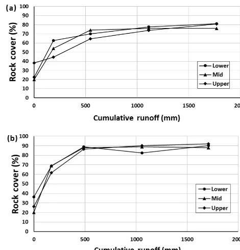
Figure 1.Plot-average rock cover (> 0.5 cm) as a function of cumu-lative runoff for the six experiments.

roughness measurements. The velocity measurements were made near the end of each simulation (and toward the begin-ning of the first simulation), so the values of the rock cover and roughness were very nearly the same as the values mea-sured at the end of each simulation (or prior to the first), but were adjusted slightly based on the measurements of rock cover and roughness that were made at the end of the pre-vious simulation (or prior to the simulation, in the case of simulation 1.)

Random roughness was calculated as the standard devia-tion of all the trend-adjusted elevadevia-tion measurements from the laser distance meter after removing 10 cm of data from the edges of the plot to remove plot edge effects.

3 Results

3.1 Rock cover and random roughness evolution The initial rock covers for the six experiments ranged from 16 to 40 %, and final covers ranged from 78 to 90 % (Fig. 1). There was no relationship between the final rock cover and either the slope gradient (Table 1) or the initial rock cover (Fig. 1). Increasing the threshold size for defining “rock” from 0.5 cm to 1 and 2 cm did not change this result. There were also no trends in final rock cover as a function of the dis-tance down the plot (Table 1), and there were no consistent trends in the rate of rock cover development as a function of downslope distance (Fig. 2). An example photo of rock cover taken after simulation 3 at 20 % slope, replication 2, is shown in the Supplement.

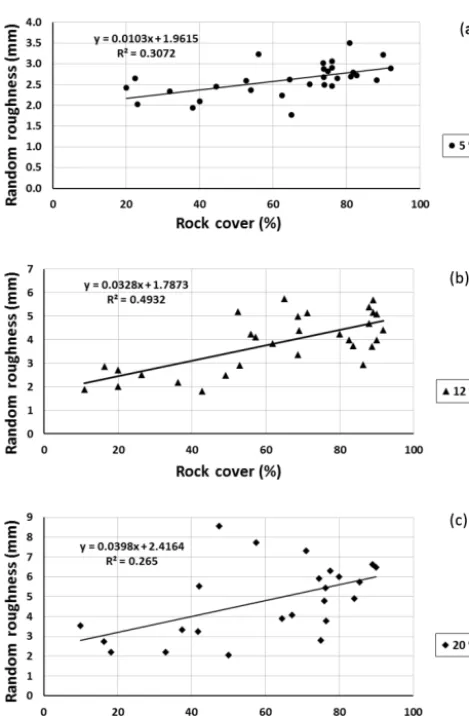
The final random roughness was quite different as a func-tion of slope gradient treatments, with the steeper slopes re-sulting in a rougher final surface (Table 1, Fig. 3). There were no consistent differences in random roughness mea-sured in the lower, middle, and upper sections of the plots (e.g., Fig. 4).

Table 1.Percentages of rock cover greater than 0.5 cm for the full, lower, middle, and upper portions of the plots, and laser-measured random roughness measured at the end of each experimental repli-cation.

Slope Rep Rock cover Random Full Lower Middle Upper Roughness

% % % % % mm

5 1 89 90 92 88 2.90 2 80 81 76 81 3.04

12 1 85 80 89 84 4.39 2 90 90 88 92 4.97

20 1 78 78 80 75 6.08 2 88 90 89 85 6.29

3.2 Runoff velocity and hydraulic friction evolution Measured runoff velocities tended to decrease as the slopes evolved to relatively consistent values of approximately 0.035 to 0.04 m s−1_{at 59 mm h}−1_{rainfall intensity, and 0.55} to 0.7 m s−1at 178 mm h−1rainfall intensity (Fig. 6). Veloci-ties on the evolved plots (at the end of the experiments) were independent of slope gradient. The results support the hy-pothesis that flow velocities are dependent on overland flow unit discharge independent of slope gradient (Fig. 7), and the results fit a power relationship well:

v=26.39q0.696 (r2=0.95, n=36), (3) wherevis the average flow velocity (m s−1) andqis the unit flow discharge across the plot (m2s−1_{). Note that the flow} variable used here is unit discharge, with units of (m2s−1_), rather than total discharge, which has units of (m3s−1), which has been used in many previous studies of rill flow velocity.

Corresponding to the changes in runoff velocities, hy-draulic friction factors indicated an increase in hyhy-draulic roughness as the surfaces evolved (Fig. 8). By the time that cumulative runoff reached 1000 mm, according to the Chezy and Manning coefficients, the surfaces were hydraulically rougher on the steeper slopes (i.e., Chezy values were less and Manning values greater on steeper slopes compared to shallower slopes). Also, Chezy and Manning coefficients were different for the two rainfall intensities (and hence runoff rates), with lesser Chezy values and greater Manning values (e.g., apparently hydraulically rougher) for the lower rainfall and runoff rates. These results were statistically sig-nificant.

3.3 Hydraulic and physical surface roughness

There were very clear and strong relationships between the hydraulic roughness coefficients (Manning and Chezy) and measured random roughness from the laser measurements

Figure 2.Surface rock cover (> 5 mm) on the three sections of the plots as a function of cumulative runoff for(a)5 % slope, replication 2, and(b)12 % slope, replication 2.

Figure 3.Averages of the three cross-section (lower, middle, and upper) laser-measured random roughness measurements (mm) as a function of cumulative runoff for the six experiments.

Figure 4.Laser-measured random roughness measurements (mm) at the three cross sections (lower, middle, and upper) as a function of cumulative runoff at 5 % slope, replications 1 and 2.

Figure 5.Random roughness as a function of rock cover on all sec-tions of the plots and both replicasec-tions for(a)5 %,(b)12 %, and(c) 20 % slope gradients.

4 Discussion

Our results that show no dependence of final rock cover per-centages, after the development of the erosion pavements, as a function of slope gradient (Fig. 1, Table 1) appear to

con-Figure 6.Flow velocities down the full plot as a function of cumu-lative runoff depth for(a)I=59 mm h−1and(b)I=178 mm h−1.

tradict previous findings that indicate greater rock cover on steeper slopes. However, the final rock covers measured in this experiment are greater than those reported in previous work at Walnut Gulch, where the previous relationships were determined. Final rock covers in this experiment ranged from 78 % to 90 %, with an average of 85 %. Rock covers mea-sured by Simanton and Toy (1994) and Simanton et al. (1994) ranged from 2 to 77 %. We conclude from these facts that the surfaces that evolved in this experiment were at maximum or near maximum coverage possible for this soil under natural hillslope conditions and climate of the area. A possible ex-planation for the somewhat lower rock cover values on the natural hillslopes may be related to factors at work that bring new material to the surface in the natural landscape, such as bioturbation and heaving associated with freeze/thaw, both of which are active in this and many other semi-arid landscapes (Emmerich, 2003).

We are not sure yet exactly what process is taking place to effect the differences in roughness with slope independent of rock cover, but a corollary may be drawn to our understand-ing of flow rates in rills on non-rocky soils. Govers (1992) and Govers et al. (2000) reported on experiments with rills that showed a relationship between flow velocity and flow discharge independent of slope gradient on non-rocky soils. This was attributed largely to the development of headcuts (see also Rieke-Zapp et al., 2007, and Nearing et al., 1999). In our experiment it appears that development of greater form roughness occurred on the steeper slopes compared to the shallower slopes. One is tempted to compare the exponent determined from this experiment (Eq. 3) to exponents from previous work on rill flow velocities. However, it should be noted that Eq. (3) uses unit width discharge, while rill flow experiments typically reported relationships using total dis-charge (e.g., Eq. 2). Because of the complexity and variabil-ity in flow in interrill areas, it is not clear that a direct com-parison of these values is entirely valid or robust. Nonethe-less, under the specific conditions of this experiment, since width is a constant, the use of total discharge for these data would also result in an exponent of 0.696 (see Eq. 3), though the equation would have a different linear coefficient. This is greater than values previously reported for rill studies, in-cluding a value of 0.294 determined by Govers (1992), 0.459 determined by Nearing et al. (1999), and 0.39 reported by Torri et al. (2012).

Our data are not inconsistent with the hypothesis that has been proposed for channel beds, that the feedback between bed morphology, erosion, and flow velocities is associated with or controlled by the Froude number. Average Froude numbers calculated from the data tended to decrease as a function of the surface development and stabilize toward the end of the replications. Average values of the Froude number were less than one in all but two cases, both of which were measured during the early stage of the experiments when the surface was just beginning to evolve to its final state (Fig. 10). Of course there is no way of using the data presented here to know the spatial variations in the Froude number occurring on the plot at any given time, nor where the Froude num-ber may have approached unity. With detailed measurements of the surface morphology at various times during such an experiment as this, possibly combined with distributed mea-surements or modeling of the flow velocity field, it might be possible to better investigate the role of energy minimization and the Froude number threshold in the development of these types of surfaces and control of the runoff velocities.

The results of this study do not suggest that the over-land flow relationships, such as Chezy or Manning equa-tions, are physically incorrect for flow modeling, but they do suggest that there are significant practical difficulties as-sociated with their application to hillslope surfaces, which erode. Hydraulic friction factors, such as Chezy and Man-ning coefficients, are commonly used on runoff models for stony rangeland (and other) soils (Nouwakpo et al., 2016),

Figure 7.Final flow velocities for all six experiments at each of the three velocity transect measurement transects and two rainfall rates.

but this usage is problematic because the coefficients depend on slope gradient and runoff rates, and hence with distance downslope on the hill and time during the runoff event. The data clearly showed that there was no unique hydraulic co-efficient for a given surface condition. Generally, Chezy and Manning roughness coefficients are presented in tables based on surface conditions, suggesting that they are not related to either slope or runoff rates. In order to accurately implement the use of these equations in models, the coefficients used should be adjusted for slope and runoff rates, which means that they should be adjusted both temporally and spatially on a hillslope within each runoff event.

The fact that there is a unique relationship between veloc-ity and discharge would suggest that routing runoff over hill-slopes in models using such a relationship (e.g., Fig. 7) would provide more consistent and realistic results. It would appear to be counterintuitive and convoluted to apply an equation that relates velocity to flow depths and slope when the co-efficients in the equations used are dependent on slope, dis-charge rate, and physical roughness. As pointed out previ-ously with respect to flow in rills, if we assume a constant roughness coefficient, then “velocities will be over-predicted on steep slopes and under-predicted on shallower slopes” (Govers et al., 2000).

5 Summary and conclusions

Figure 8.Hydraulic friction factors, Chezy and Manning coefficients, for the full length of the plots as a function of cumulative runoff for 59 and 178 mm h−1rainfall intensities.

Figure 9.Relationships between the roughness coefficients, Chezy and Manning, to laser measured random roughness.

Velocities were dependent on discharge rates alone. The relationship between velocity and discharge was independent of slope gradient or rainfall intensity.

Use of hydraulic friction factors, such as Chezy and Man-ning coefficients, are problematic because they depend on both slope and runoff rate. The data clearly showed that there is no unique hydraulic coefficient for a given generalized sur-face condition.

Data availability. All data used in this paper are available in the Supplement.

The Supplement related to this article is available online at https://doi.org/10.5194/hess-21-3221-2017-supplement.

Competing interests. The authors declare that they have no conflict of interest.

Edited by: Roger Moussa

References

Bennett, S. J., Alonso, C. V., Prasad, S. N. and Römkens, M. J.: Experiments on headcut growth and migration in concentrated flows typical of upland areas, Water Resour. Res., 36, 1911– 1922, 2000.

Emmerich, W. E.: Season and erosion pavement influence on saturated soil hydraulic conductivity, Soil Sci., 168, 637–645, https://doi.org/10.1097/01.ss.0000090804.06903.3b, 2003. Foster, G. R., Huggins, L. F., and Meyer, L. D.: A laboratory study

of rill hydraulics: I. Velocity relationships, Trans. of the Am. Soc. Agric. Eng., 27, 790–796, 1984.

Govers, G.: Relationship between discharge, velocity and flow area for rills eroding loose, non-layered materials, Earth Surf. Proc. Landf., 17, 515–528, 1992.

Govers, G., Takken, I., and Helming, K.: Soil roughness and over-land flow, Agronomie, 20, 131–146, 2000.

Graf, W. H.: Hydraulics of Sediment Transport, Water Resources Publications, Littleton, CO, 513 pp., ISBN-0-918334-56-X, 1984.

Grant, G. E.: Critical flow constrains flow hydraulics in mobile bed streams: A new hypothesis, Water Resour. Res., 33, 349–358, 1997.

Hussein, M. H., Amien, I. M., and Kariem, T. H.: Designing ter-races for the rainfed farming region in Iraq using the RUSLE and hydraulic principles, Int. Soil and Water Conservation Res., 4, 39–44, 2016.

Lei, T., Nearing, M. A., Haghighi, K., and Bralts, V.: Rill erosion and morphological evolution: A simulation model, Water Resour. Res., 34, 3157–3168, 1998.

Nearing, M. A., Norton, L. D., Bulgakov, D. A., Larionov, G. A., West, L. T., and Dontsova, K. M.: Hydraulics and erosion in erod-ing rills, Water Resour. Res., 33, 865–876, 1997.

Nearing, M. A., Simanton, J. R., Norton, L. D., Bulygin, S. J., and Stone, J.: Soil erosion by surface water flow on a stony, semiarid 30 hillslope, Earth Surf. Proc. Land., 24, 677–686, 1999. Nearing, M. A., Norton, L. D., and Zhang, X.: Soil erosion and

sedi-mentation, in: Agricultural Nonpoint Source Pollution, edited by: Ritter, W. F. and Shirmohammadi, A., Lewis Publishers, Boca Raton, 29–58, ISBN 1-56670-222-4, 2001.

Nearing, M. A., Kimoto, A., Nichols, M. H., and Ritchie, J. C.: Spatial patterns of soil erosion and deposition in two small, semiarid watersheds, J. Geophys. Res., 110, F04020, https://doi.org/10.1029/2005JF000290, 2005.

Nouwakpo, S. K., Williams, C. J., Al-Hamdan, O., Weltz, M. A., Pierson, F., and Nearing, M. A.: A review of concentrated flow erosion processes on rangelands: fundamental understanding and knowledge gaps, Int. Soil and Water Conservation Res., 4, 75–86, 2016.

Paige, G. B., Stone, J. J., Smith, J. R., and Kennedy, J. R.: The Walnut Gulch rainfall simulator: A computer-controlled variable intensity rainfall simulator, Appl. Eng. Agric., 20, 25–34, 2004. Poesen, J. W., van Wesemael, B., Bunte, K., and Benet, A.:

Vari-ation of rock cover size along semi-arid hillslopes: a case study from Southeast Spain, Geomorphology, 23, 323–335, 1998. Rieke-Zapp, D. H., Poesen, J., and Nearing, M. A.: Effects of rock

fragments incorporated in the soil matrix on concentrated flow hydraulics and erosion, Earth Surf. Proc. Land., 32, 1063–1076, 2007.

Shaw, C. F.: Erosion Pavement, Geogr. Rev., 19, 638–641, 1929. Simanton, J. R. and Toy, T. J.: The relation between surface

rock fragment cover and semiarid hillslope profile morphology, Catena, 23, 213–225, 1994.

Simanton, J. R., Renard, K. G., Christiansen, C. M., and Lane, L. J.: Spatial distribution of surface rock fragments along catenas in semiarid Arizona and Nevada, USA, Catena, 23, 29–42, 1994. Stone, J. J. and Paige, G. B.: Variable rainfall intensity rainfall

simu-lator experiments on semi-arid rangelands, Proc. 1st Interagency Conf. on Res. in the Watersheds, Benson, AZ, USA, 27–30 Oc-tober 2003, 83–88, 2003.

Takken, I., Govers, G., Ciesiolka, C. A. A., Silburn, D. M., and Loch, R. J.: Factors influencing the velocity-discharge relation-ship in rills, in: Modelling Soil Erosion, Sediment Transport and Closely Related Hydrological Processes, IAHS Publ. no. 249, 63–70, 1998.

Torri, D., Poesen, J., Borselli, L., Bryan, R., and Rossi, M.: Spatial variation of bed roughness in eroding rills and gullies, Catena, 90, 76–86, 2012.