Validation of terrestrial water storage variations as simulated by different global numerical models with GRACE satellite observations

www.hydrol-earth-syst-sci.net/21/821/2017/ doi:10.5194/hess-21-821-2017

© Author(s) 2017. CC Attribution 3.0 License.

Validation of terrestrial water storage variations as simulated by

different global numerical models with GRACE satellite

observations

Liangjing Zhang1, Henryk Dobslaw1, Tobias Stacke2, Andreas Güntner1, Robert Dill1, and Maik Thomas1,3 1_{Helmholtz Centre Potsdam, GFZ German Research Centre for Geosciences, 14473 Potsdam, Germany}

2_{Max Planck Institute for Meteorology, Hamburg, Germany}

3_{Institute of Meteorology, Free University of Berlin, Berlin, Germany}

Correspondence to:Liangjing Zhang ([email protected]) Received: 29 June 2016 – Discussion started: 22 July 2016

Revised: 5 December 2016 – Accepted: 18 January 2017 – Published: 10 February 2017

Abstract.Estimates of terrestrial water storage (TWS) vari-ations from the Gravity Recovery and Climate Experiment (GRACE) satellite mission are used to assess the accuracy of four global numerical model realizations that simulate the continental branch of the global water cycle. Based on four different validation metrics, we demonstrate that for the 31 largest discharge basins worldwide all model runs agree with the observations to a very limited degree only, together with large spreads among the models themselves. Since we ap-ply a common atmospheric forcing data set to all hydrologi-cal models considered, we conclude that those discrepancies are not entirely related to uncertainties in meteorologic in-put, but instead to the model structure and parametrization, and in particular to the representation of individual storage components with different spatial characteristics in each of the models. TWS as monitored by the GRACE mission is therefore a valuable validation data set for global numerical simulations of the terrestrial water storage since it is sensitive to very different model physics in individual basins, which offers helpful insight to modellers for the future improve-ment of large-scale numerical models of the global terrestrial water cycle.

1 Introduction

Global Soil Wetness Project (GSWP; Dirmeyer et al., 2006; Dirmeyer, 2011), the Water Model Intercomparison Project (WaterMIP; Haddeland et al., 2011), and the Inter-Sectoral Impact Model Intercomparison Project (ISI-MPI; Schewe et al., 2014), which compare the results from a multitude of models to highlight shortcomings and inconsistencies. These projects have primarily focused on evapotranspiration or soil moisture content. Gudmundsson et al. (2012) have also eval-uated nine large-scale hydrological models based on runoff observations.

The terrestrial water storage (TWS), which is understood here to contain all water components stored above and un-derneath the land surface, including soil moisture, the water content of snowpack, land ice, surface water, and groundwa-ter in shallow and deep aquifers, forms an important com-ponent of the terrestrial water cycle. It is difficult to di-rectly measure TWS on the ground due to insufficient in situ observations of the very diverse hydrological stores and fluxes. The terrestrial water budget method estimates TWS by solving the terrestrial water balance equation through the data of precipitation, runoff and evapotranspiration from ob-servations and atmospheric reanalysis (Zeng et al., 2008; Tang et al., 2010; Rodell et al., 2011), while TWS varia-tions can also be derived from combined atmospheric and ter-restrial water-balance computations, utilizing water vapour content and moisture flux convergence from atmospheric re-analysis data and river discharge measurements (Seneviratne et al., 2004; Hirschi et al., 2006). However, these methods are highly dependent on the accuracy of the reanalysis data, which often contain systematic errors, in particular at inter-annual timescales and longer. The Gravity Recovery and Climate Experiment (GRACE) launched in 2002 provides a unique data source to estimate spatio-temporal variations of the Earth’s water storage at regional up to global scales (Ta-pley et al., 2004; Wahr et al., 2004). Averaged over an arbi-trary area with a spatial extent of 100 000 km2 and greater, TWS derived from GRACE is believed to reach an accuracy of better than 1 cm equivalent water thickness (Dahle et al., 2014). Although there is a mismatch between the spatial res-olution of GRACE data and that of hydrological models, the effective spatial resolution can be extrapolated to finer spatial scales through proper post-processing (Landerer and Swen-son, 2012). There are now more than 13 years of GRACE data available and this length of the time series together with a recently completed reprocessing of the whole GRACE record (Dahle et al., 2012) motivates us to revisit the question of what can be learned from GRACE on the performance of global hydrological models in representing continental water storage variations.

Through the comparison of basin-averaged TWS from models with GRACE-based estimates, we intend to iden-tify the advantages and deficiencies of a certain model and analyse the reasons for different model behaviours. Globally gridded TWS variations and uncertainties from GRACE es-timated by the same post-processing procedure as described

by Zhang et al. (2016) are applied. We quantitatively analyse the correspondence between TWS estimates from four avail-able hydrological models and GRACE in 31 of the world’s largest river basins. To separate the effects of atmospheric in-put data, all the models apply the same meteorological forc-ing data set. Actual evapotranspiration and runoff rates cal-culated with the different models are also analysed. Consid-ering the diversity of the performance of the models in these 31 basins, we focus on time series of TWS variations in two regions which are characterized by different climate regimes, i.e. the snow-dominated catchments and the dry catchments, by looking into the TWS variation time series from models and GRACE. In addition, snow, surface water and subsurface water including root zone and/or deep layer storage from the models are also compared in order to analyse the contribution of different storage components to the total water storage. By investigating the relative performance of these different mod-els, we intend to contribute to the future model development of both LSMs and GHMs.

2 Data set

2.1 Hydrological model simulations

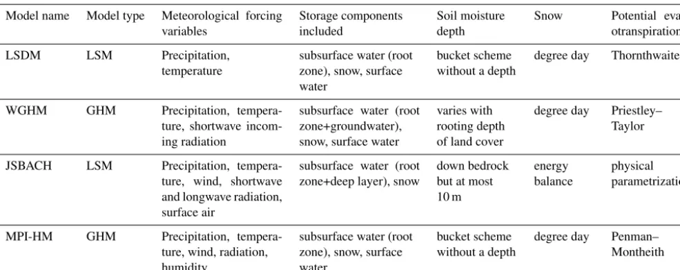
For this study, we selected four different models to repre-sent a broad range from conceptual hydrological to complex land surface models (Table 1). In order to ensure that this spread between the simulations is indeed related to the differ-ent represdiffer-entation of physics in the model, all the models are forced with the WFDEI data set based on ERA-Interim re-analysis data (Dee et al., 2011) that has been developed dur-ing the WATCH project (Weedon et al., 2011). This WFDEI meteorological forcing data set is a quasi-observation which combines the daily variability of the ERA-Interim re-analysis with monthly in situ observations such as temperature and precipitation (Weedon et al., 2014). There are two precipi-tation products available from WFDEI: (1) corrected by us-ing the Climate Research Unit at the University of East An-glia (CRU) observations; and (2) corrected with the Global Precipitation Climatology Centre (GPCC) data set. Since the WFDEI data sets incorporating the CRU-based precipitation products cover a longer time span, they are used in our study and referred to subsequently as WFDEI-CRU.

ver-Table 1.Overview of the main characteristics of the four numerical models particularly considered in this study.

Model name Model type Meteorological forcing variables

Storage components included

Soil moisture depth

Snow Potential evap-otranspiration

LSDM LSM Precipitation,

temperature

subsurface water (root zone), snow, surface water

bucket scheme without a depth

degree day Thornthwaite

WGHM GHM Precipitation,

tempera-ture, shortwave incom-ing radiation

subsurface water (root zone+groundwater), snow, surface water

varies with rooting depth of land cover

degree day Priestley– Taylor

JSBACH LSM Precipitation, tempera-ture, wind, shortwave and longwave radiation, surface air

subsurface water (root zone+deep layer), snow

down bedrock but at most 10 m

energy balance

physical parametrization

MPI-HM GHM Precipitation, tempera-ture, wind, radiation, humidity

subsurface water (root zone), snow, surface water

bucket scheme without a depth

degree day Penman– Montheith

sion of WGHM as calibrated for WFDEI-GPCC forcing (ver-sion 2.2 STANDARD; Müller Schmied et al., 2014) is used in this study. However, we run the model with WFDEI-CRU forcing without re-calibration.

The Land Surface Discharge Model (LSDM; Dill, 2008) is based on the Simplified Land Surface Scheme (SL-Scheme) and the Hydrological Discharge Model (HD-Model; Hage-mann and Gates, 2003, 2001) from the Max Planck Institute for Meteorology. The global water storage variations contain surface water in rivers, lakes and wetlands, groundwater and soil moisture, as well as water stored in snow and ice. The code has been tailored to enable the simulation of continen-tal water mass redistribution for geodetic applications that include the derivation of effective angular momentum func-tions of the continental hydrosphere to interpret and predict changes in the Earth’s rotation (Dobslaw et al., 2010; Dill and Dobslaw, 2010), and of vertical crustal deformations as observed from GPS permanent stations (Dill and Dobslaw, 2013).

JSBACH (Raddatz et al., 2007; Brovkin et al., 2009) is a land surface model and forms together with ECHAM6 (Stevens et al., 2013) and MPIOM (Jungclaus et al., 2013) the current Max Planck Institute for Meteorology’s Earth System Model (MPI-ESM). As part of the MPI-ESM, JS-BACH includes interactive vegetation and a five-layer soil hydrology scheme to provide the lower atmospheric bound-ary conditions over land, particularly the fluxes of energy, water and momentum. For this study, however, JSBACH was used in an offline mode without interactive coupling to the other MPI-ESM components, but driven by prescribed WFDEI-CRU atmospheric forcing. Snow in JSBACH is treated as external layers above the soil column, with a max-imum of five snow layers. Soil moisture in deep layers below

the root zone is simulated and buffers extreme soil moisture conditions in the layers above.

Finally, the Max Planck Institute of Meteorology’s Hy-drology Model (MPI-HM; Stacke and Hagemann, 2012) is a global hydrological model. Its water flux computations are of similar complexity to land surface models, but it does not account for any energy fluxes. In addition to precipitation and temperature, it requires potential evapotranspiration as input which also was derived from the WFDEI using the Penman– Montheith equation, similarly to the Weedon et al. (2011) study. TWS from MPI-HM is simulated as the sum of soil moisture in the root zone, snow and surface water.

Some of the main characteristics of the four numerical models are presented in Table 1, which provide more in-formation on how models are different from each other. For instance, although soil moisture and snow water are in-cluded in all the models, surface water and groundwater are simulated differently. JSBACH is the only model which does not include surface water. Groundwater is simulated by WGHM, where the anthropogenic impact such as ground-water abstraction is also considered. JSBACH does not sim-ulate groundwater directly but includes the subsurface wa-ter in the deep layer, whereas groundwawa-ter is not considered by the other two models. We use the term subsurface water for both soil moisture and groundwater. But the impact from consideration of groundwater to TWS variations will be in-vestigated in the following discussion.

LSDM, WGHM and MPI-HM are provided on a 0.5◦_by

averaged over the selected basins to obtain the basin-scale TWS. Since ice dynamics and glacier mass balance are not included in the numerical models applied in this study, water mass variations in Antarctic and Greenland are not consid-ered throughout the reminder of this paper.

2.2 TWS estimates from GRACE

The GRACE US–German twin satellite mission provides es-timates of month-to-month changes in the gravitational field of the Earth mainly based on precise K-band microwave measurements of the distance between two low-flying satel-lites (Wahr, 2009) since April 2002. After correcting for short-term variability due to tides in the atmosphere (Bian-cale and Bode, 2006), solid Earth (Petit and Luzum, 2010) and oceans (Savcenko and Bosch, 2012), as well as due to non-tidal variability in the atmosphere and oceans (Dob-slaw et al., 2013) from the observations, the resulting gravity changes mainly represent mass transport phenomena in the Earth system, which are – apart from long-term trends – al-most exclusively related to the global water cycle.

We use the monthly GRACE release 05a Level-2 prod-ucts from GFZ Potsdam (Dahle et al., 2012), which can be downloaded from the website of the International Cen-tre for Global Earth Models (http://icgem.gfz-potsdam.de/ ICGEM). The GRACE products are expressed in terms of fully normalized spherical harmonic (SH) coefficients up to degree and order 90, approximately corresponding to a global resolution of 2◦ in latitude and longitude. We apply the same post-processing steps to the GRACE data as de-scribed by Zhang et al. (2016). The degree-1 coefficients are added following the method of Bergmann-Wolf et al. (2014). The non-isotropic filter DDK2 corresponding to an isotropic Gaussian filter with 680 km full width half maxi-mum (Kusche, 2007; Kusche et al., 2009) is applied to re-move correlated errors at particular higher degrees of the spherical harmonic expansion. In order to account for sig-nal attenuation and leakage caused by smoothing and fil-tering, local re-scaling factors are introduced for each grid cell. We use median re-scaling factors obtained from a small ensemble of global hydrological models. The gridded TWS anomalies are then estimated which can be averaged over arbitrary basins. As for the model data, the linear trend is removed over the period January 2003 to December 2012. Error estimates as a quadrature of measurement error, leak-age error and re-scaling error are also provided to assess the signal-to-noise ratio (SNR) of GRACE for particular basins (full details are given in Zhang et al., 2016). In the case of a small signal-to-noise ratio, discrepancies between TWS from GRACE and models might also be attributed to compara-tively large GRACE TWS errors.

Figure 1.Locations of 31 globally distributed basins from the sim-ulated topological networks (STN-30p) with underlying Köppen– Geiger climate zones. Basin IDs and names are indicated in Table 2.

3 Evaluation of TWS from model realizations with GRACE

We compare the basin-averaged TWS from GRACE with the results of four different numerical model realizations intro-duced above. In total, 31 globally distributed basins where the GRACE SNR is larger than 2 (see Fig. 1 and Table 2) are selected for further study. We first focus on the global statistical performance of the models compared to GRACE. For these basins, evaluation metrics as suggested by Gud-mundsson et al. (2012) that focus both on seasonal signals and year-to-year variability are applied.

3.1 Evaluation metrics

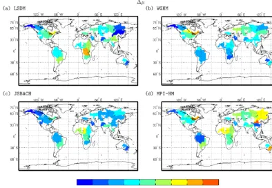
First, relative annual amplitude differences are calculated ac-cording to

1µ=(µM−µO)/µO, (1)

whereµOis the annual amplitude of the time series of TWS variations from GRACE, and µM the annual TWS ampli-tudes from the different model realizations (Fig. 2). Second, the timing of the annual cycle is assessed using phase dif-ferences of the annual harmonic for models and observations according to

1φ=φM−φO. (2)

If the value of1φ is negative, it implies that the seasonal maximum is earlier in the year in the model than in GRACE (Fig. 3). Annual amplitude and phase are calculated by least square regression as follows:

MIN=! (1TWS(t )−(Asin(2π t /T+φ))T(1TWS(t ) (3) −(Asin(2π t /T+φ)),

Figure 2.Relative amplitude differences of four hydrological model realizations with GRACE-based TWS observations.

Figure 4.Variance of GRACE-based TWS observations that is explained by TWS as simulated in four hydrological model realizations.

model realizations are calculated:

R2=(var(TWSO)−var(TWSO−TWSM))/var(TWSO), (4) where var denotes the variance operator. Fourth, we repeat the calculation of the explained variances for TWS time se-ries from GRACE and the models with the mean seasonal variability removed.

3.2 Global evaluation

As shown in Fig. 2, the values of 1µfor WGHM and JS-BACH are mostly negative. For JSJS-BACH, these negative val-ues mainly occur at mid to high latitudes of the Northern Hemisphere. WGHM underestimates the annual amplitude, especially at the low latitudes. Contrarily, MPI-HM has more basins with positive 1µ. For LSDM, most 1µ values lie between −0.3 and 0.3, indicating on average better agree-ment of annual amplitude with GRACE. The phase differ-ence varies more among the different models, but in most cases an earlier seasonal storage maximum is shown for the model runs relative to GRACE. There are more basins with phase difference values near zero for LSDM, while WGHM, JSBACH and MPI-HM show large differences with respect to the GRACE result, especially at high latitudes of the Northern Hemisphere (Fig. 3). LSDM explains the GRACE TWS variations relatively better than the other models at most basins (Fig. 4). Only in the Yukon, Nile, Zaire, Yangtze, Indus and the two basins in Australia are explained variances less than 50 %. Low values of explained variance also occur at the mid-latitude of the Northern Hemisphere for WGHM. JSBACH and MPI-HM perform generally better at basins in Africa, but have worse results in Siberia. When the annual signal is removed, the explained variances for TWS time se-ries from GRACE and the models are generally less than 60 % (Fig. 5), indicating the models’s poor ability to cap-ture the inter-annual variations. LSDM shows especially low explained variance values for many basins in Africa.

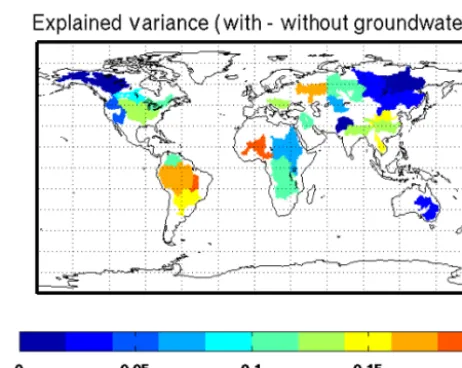
The impact from consideration of groundwater to TWS variations in WGHM is investigated by showing the differ-ences of explained variances with and without groundwa-ter (Fig. 6). The positive values indicate that WGHM with groundwater exhibits better agreement with GRACE than the one without. The large impact is mainly located at basins such as Tocantins, Niger, Huang He, Mekong and Missis-sippi. Only in three basins (Lena, Indus and Yukon) is the effect of groundwater consideration on the model negative.

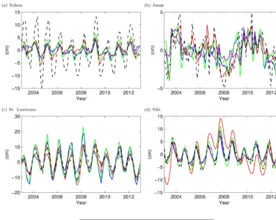
As each metric usually focuses only on one specific prop-erty of statistical performance and has its own limitations, the time series of TWS are given for some basins with the largest deviation between GRACE and the model. We show the Yukon basin, where both WGHM and JSBACH exhibit the largest deviation of annual amplitudes from GRACE. Although the annual amplitude is simulated bet-ter by LSDM and MPI-HM, apparent negative phase differ-ences are shown. The Amur basin is also shown, as LSDM,

Figure 6.The differences between the explained variance values from WGHM with and without groundwater.

WGHM and MPI-HM all have the largest negative phase dif-ferences with GRACE here. Models generally capture the inter-annual signals but perform quite differently among each other and with GRACE in terms of seasonality. Almost op-posite phase differences are found for these models. The smallest explained variance for MPI-HM happens at the St. Lawrence basin, where a much larger amplitude and a neg-ative phase difference compared with GRACE are found. When the annual signal is removed, models perform differ-ently in terms of the explained variance. In the Nile basin, large inter-annual variations simulated by LSDM even lead to negative explained variance compared with the other mod-els.

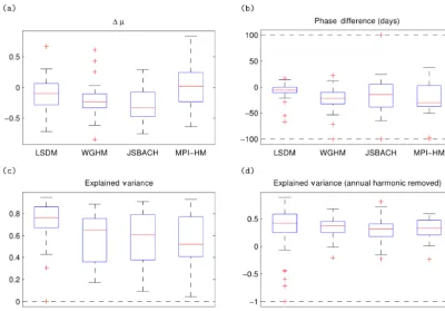
Figure 8 summarizes the overall performance of each sta-tistical metric for all the basins considered by means of box plots. The median1µfor MPI-HM is almost zero where the other three values are all negative, indicating an underestima-tion of the annual amplitude of TWS from LSDM, WGHM and JSBACH. As shown in Fig. 2d, MPI-HM overestimates the TWS variations at many basins, which compensate with those underestimated values and lead to a median value at al-most zero. All the models have a median phase difference be-low zero, with LSDM having the smallest bias and range, and MPI-HM the largest bias. This means that the TWS peaks of the models tend to proceed GRACE peaks. For the explained variance, LSDM shows the best median value, followed by WGHM, JSBACH and MPI-HM. However, when the annual signal is removed, many outliers appear in LSDM for the ex-plained variances, while WGHM and MPI-HM show slightly better performances.

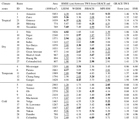
Table 2.Characteristics of the basins shown in Fig. 1. Bold and underlined numbers are the largest and smallest rms differences between GRACE and models separately.

Climate Basin Area RMSE (cm) between TWS from GRACE and GRACE TWS

zones ID Name (1000 km2) LSDM WGHM JSBACH MPI-HM Error (cm) SNR

Tropical

1 Amazon 5853 4.39 6.08 5.60 9.53 1.46 9.76

3 Zaire 3699 5.26 3.36 3.08 3.49 1.32 3.82

21 Orinoco 1039 6.37 4.96 6.21 5.79 3.14 4.74

29 Mekong 774 5.87 5.60 6.28 4.51 3.86 3.73

30 Tocantins 769 7.69 7.49 4.99 5.45 2.81 5.95

Dry

2 Nile 3826 4.02 1.85 1.61 1.39 1.06 3.26

10 Niger 2240 2.53 2.97 1.87 2.23 1.29 4.93

15 Chari 1571 2.94 1.96 2.40 2.50 1.50 3.42

18 Indus 1143 2.17 2.61 3.08 3.04 1.54 2.42

19 Syr-Darya 1070 2.00 3.30 3.07 2.89 1.12 3.65

22 Murray 1031 3.45 3.61 3.68 3.38 1.88 2.73

23 Great Artesian 977 2.44 2.67 2.36 2.22 1.33 2.67

24 Shatt el Arab 967 2.28 3.64 3.67 2.85 1.49 3.81

25 Huang He 894 1.52 2.09 1.74 2.38 1.28 2.35

27 Colorado(Ari) 807 1.90 2.59 2.98 2.91 1.41 2.78

Temperate

4 Mississippi 3203 1.68 3.54 2.36 3.45 0.86 6.60

6 Parana 2661 4.17 3.03 3.59 2.81 1.32 4.50

11 Zambezi 1989 2.89 7.05 4.83 3.30 1.57 6.80

12 Chang Jiang 1794 2.58 2.05 3.24 3.12 1.49 3.09

14 Ganges 1628 4.04 4.43 3.73 2.90 1.94 5.99

Cold

5 Amur 2903 1.20 1.73 1.88 2.05 0.68 3.18

7 Yenisei 2582 1.89 2.34 3.44 3.54 0.68 6.67

8 Ob 2570 1.50 3.20 4.35 4.14 0.68 8.31

9 Lena 2418 2.33 2.40 3.40 3.99 0.68 6.01

13 Mackenzie 1713 2.67 2.83 3.95 3.39 0.83 6.20

16 Volga 1463 2.11 4.55 3.28 5.22 0.84 8.43

17 St. Lawrence 1267 2.59 4.74 3.42 4.88 1.14 4.94

20 Nelson 1047 1.67 3.87 3.19 3.31 1.12 3.82

26 Yukon 852 5.06 5.72 5.74 5.29 1.19 7.68

28 Danube 788 1.72 4.18 4.03 4.27 1.50 4.96

31 Columbia 724 2.69 4.75 6.09 5.71 1.85 5.32

basins are grouped according to the Köppen climate zones (Kottek et al., 2006), which include tropical climates, dry cli-mates, temperate climates and cold climates (see Fig. 1). For most of the basins, the GRACE errors are much smaller than the rms differences, which indicates that the main contribu-tions to the differences arise from model uncertainties. Out of the five basins in the tropical zone, three basins have the largest differences between TWS variations from GRACE and models in LSDM. In contrast, WGHM has no largest differences in this climate zone. The smallest value, how-ever, seems to occur randomly among the models. In the dry zone, most basins have low SNR values and the small-est rms of the TWS differences is sometimes quite close to the GRACE TWS errors. For instance, at basins like the Nile, Indus, and the two Australian basins, the GRACE SNR estimates are all below 3. Thus, it is likely that the large

uncertainty in GRACE TWS estimates contributes largely to the bad agreement in these basins. Still, MPI-HM and LSDM perform comparably better, showing a smaller num-ber of largest differences and comparably more smallest dif-ferences. In the temperate zone, WGHM has the most largest differences, while MPI-HM has the least. There is, however, no regular pattern of where the smallest difference occurs. In the cold zone, all the smallest differences happen in LSDM, whereas the largest differences mainly occur at MPI-HM and JSBACH.

cli-Figure 7.Examples of monthly TWS time series from GRACE and models for the basins with the largest deviation between model and GRACE in each of the four metrics: relative amplitude differences (Yukon), phase differences (Amur), explained variance (St. Lawrence) and explained variance with annual harmonic signal removed (Nile).

mates in more detail. There, we assess actual evapotranspi-ration (AET) and runoff which are the main components of the terrestrial water budget and subsequently look into the mean monthly time series of TWS and its individual storage components.

3.3 Actual evapotranspiration and runoff

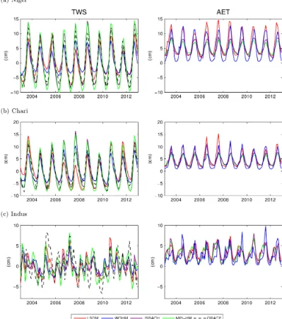
As part of the terrestrial branch of the water cycle, actual evapotranspiration (AET) and runoff may explain part of the differences among the models in terms of storage variations. Although some large differences of AET are present, the effects on subsequently simulated TWS are damped. Espe-cially in humid areas, no direct impact can be found. For arid basins, however, the impact from AET is more dominant. We choose three particularly affected basins (Niger, Chari and Indus) and show the AET time series from all models (Fig. 9). For these basins, the time series comparison shows that the smaller (or larger) AET in the wet season leads to higher (or lower) seasonal amplitude of TWS. In addition, in these dry areas, LSDM generally exhibits enhanced AET due to high temperatures and extremely low humidity which then lead to smaller TWS variations. As exemplarily

demon-strated for the Niger basin, the relatively larger AET from LSDM covering the time period 2007 to 2009 is just corre-spondent to the comparably smaller TWS variations. AET is calculated from the potential evapotranspiration (PET) as a function of the available amount of water. While starting with the same meteorological forcing data, PET is calculated differently by the models using various approaches. PET in the LSDM is calculated by the Thornthwait method, using only the daily temperature and a seasonal heat index that is based on monthly mean temperatures. In WGHM, PET is based on the Priestley–Taylor approach using net radiation, which in turn is computed as a function of incoming short-wave radiation, temperature and surface albedo. For MPI-HM, PET is computed in a pre-processing step based on Penman–Montheith using radiation, temperature, wind and humidity. JSBACH computes evaporation based on the en-ergy balance by internally computing atmospheric water de-mand.

Figure 8.Box plots illustrating the1µ(a), phase differences(b), explained variance and(c)explained variance with the annual harmonic signal removed(d)for the TWS from GRACE and models. The red horizontal line is the median, the edges of the box are the 25th and 75th percentiles, the whiskers extend to the most extreme data points not considered outliers, and outliers are plotted individually and set within the extreme data limits as indicated by the dashed line.

models following the equation

R(t )=P (t )−ET(t )−TWSC(t ), (5) wheretis the time,P, ET andRare the basin-averaged pre-cipitation, evapotranspiration and runoff, and TWSC is the terrestrial water storage change (Ramillien et al., 2006). It is seen that the performance of a certain model is connected with its differently simulated runoff. At the Amazon basin, the comparably large runoff simulated from MPI-HM also leads to smaller variability in TWS, which is also shown at the Orinoco basin. At the Mekong basin, the larger amplitude in TWS from JSBACH compared with GRACE is related to the apparently small amplitude in its runoff.

3.4 Snow-dominated catchments

As highlighted in Sect. 3.2, models perform quite differently at high latitudes of the Northern Hemisphere (cold zone), which are generally dominated by snow. Especially JSBACH and MPI-HM show large differences in the TWS when com-pared with GRACE. We focus here on four basins in this area, Lena, Yenisei, Ob and Yukon, and look into the mean monthly time series of the TWS and its different components (Fig. 11). For LSDM and MPI-HM, subsurface water only in-cludes the water storage in the root zone, while for WGHM

Figure 9.Time series of TWS (left) from GRACE and models and model-simulated AET time series (right), each for three different catch-ments in the dry zone: Niger, Chari, and Indus.

scheme applied by JSBACH. Yukon, however, is quite dif-ferent from the other snow-dominated basins. Here, all the models underestimate the annual amplitude of TWS when compared with GRACE. Since the basin-average TWS er-ror from GRACE at Yukon is 1.19 cm and much smaller than the discrepancies between GRACE and the models (Table 2), it could be the case that all models fail to represent certain hydrological processes, or that our GRACE TWS errors are too optimistic here since the re-scaling errors are also esti-mated from a hydrological model ensemble. In addition, Seo et al. (2006) found also large TWS errors at Yukon basin and

suggested that the atmosphere and ocean tidal and non-tidal de-aliasing errors might be a problem in this area. Investigat-ing those discrepancies in full detail, however, is beyond the scope of our present paper and will be left open for future study.

3.5 Dry catchments

Figure 10. Time series of TWS (left) from GRACE and models and model-simulated runoff time series (right), each for three different catchments in the tropical zone: Amazon, Orinoco, and Mekong.

contributor to the TWS changes (Fig. 12). The TWS varia-tions from JSBACH and MPI-HM show a quite similar an-nual cycle when compared to GRACE. MPI-HM generally exhibits a larger amplitude in simulated subsurface water and TWS. WGHM deviates considerably with a much smaller amplitude and a large phase shift in the subsurface water. The simulated surface water from WGHM brings TWS slightly closer to that from GRACE. LSDM, however, performs dif-ferently in these two basins. In the Nile basin, although the subsurface water from LSDM is consistent with JSBACH and MPI-HM, the simulated surface water variations lead to a higher amplitude of TWS variations when compared with

Figure 11.Mean monthly time series of TWS (first column) and the individual storage contributions from subsurface water (second column), snow water equivalent (third column) and surface water (fourth column), each for four snowy catchments: Ob, Lena, Yenizei and Yukon. TWS from GRACE (dashed line) has been included in every sub-figure for reference.

snow variations properly. MPI-HM performs poorly in sim-ulating the surface water, with a delayed dynamics which leads to a preceded annual cycle. At the Huang He basin, the subsurface water from LSDM, WGHM and JSBACH as the main contributors to the TWS show similar annual vari-ations to GRACE, while MPI-HM has a much larger ampli-tude. The surface water, however, is simulated differently by LSDM and WGHM, which consequently leads to different TWS variations.

4 Summary

Figure 12.Mean monthly time series of TWS (first column) and the individual storage contributions from subsurface water (second column), snow water equivalent (third column) and surface water (fourth column), each for four dry catchments: Nile, Niger, Indus and Huang He. TWS from GRACE (black line) has been included in every sub-figure for reference.

At certain basins like the Danube, Tocantins, Columbia, Ganges, Mekong, and Amazon, all numerical models show good agreement with GRACE. However, models still per-form quite differently at many other basins, even though forced with the same meteorological data set. At the Nile, Indus, Murray and Great Artesian basins, large TWS errors and low SNR are found, which suggests a major contribution from GRACE errors to the differences. A good capture of annual amplitude and phase at most basins leads to high val-ues of explained variance in many basins for LSDM. How-ever, serious problems are also found in the same model run in some central Africa basins, like the Nile and Zaire, where TWS simulated by LSDM exhibits unusual large inter-annual

variations. WGHM performs generally well in tropical and cold regions, but rather poorly in the temperate zone. JS-BACH and MPI-HM show large discrepancies with GRACE at the basins at high latitudes of the Northern Hemisphere.

com-ponent, the simulated snow variations in JSBACH already show smaller amplitude and negative phase differences com-pared with all the other models. This could be related to the fact that JSBACH simulates snow in a more physical way based on energy balance, which is totally different from the degree-day method applied by all the other models. The comparably better agreement of LSDM and WGHM with GRACE in terms of TWS in these snow-dominated basins is partly caused by the realistic surface water component rep-resented by these two models. In the dry catchments, the im-pact from AET on TWS is relatively strong. The smaller AET from MPI-HM also leads to better agreement with GRACE, whereas LSDM shows large differences with GRACE in terms of TWS, especially at some dry basins in central Africa, partly due to the overly simple evaporation scheme. PET is simulated using a superior parametrization by MPI-HM, while LSDM still applies the traditional Thornthwaite method based solely on air temperature. The groundwater considered by WGHM also has some impact on the simu-lated TWS, especially at basins such as Tocantins, Mekong, Niger and Mississippi. At the Yukon basin, we found the bad performance of all models in terms of TWS when compared with GRACE, which could be due to the effects of atmo-spheric and oceanic de-aliasing errors not further discussed in our current study. In future, we would like to assess all pos-sible errors of GRACE TWS through investigation of simu-lated GRACE-type gravity field time series (Flechtner et al., 2016) based on realistic orbits and instrument error assump-tions as well as background error assumpassump-tions out of the up-dated ESA Earth system model (Dobslaw et al., 2015, 2016), which we believe will further help to explain the discrep-ancy between global models of the terrestrial water cycle and GRACE satellite observations.

5 Data availability

GRACE data at different processing levels are publicly available via ftp://isdcftp.gfz-potsdam.de/grace/ (Dahle et al., 2012). Post-processed TWS data based on GRACE sensor data are moreover accessible via the interac-tive web interface http://icgem.gfz-potsdam.de/ICGEM/JSB/ G3Browser-st.html (Zhang et al., 2016).

Competing interests. The authors declare that they have no conflict of interest.

Acknowledgements. This study has been supported by the German Federal Ministry of Education and Research within the FONA research program under grants 03F0654A and 01LP1151A.

The article processing charges for this open-access publication were covered by a Research

Centre of the Helmholtz Association.

Edited by: W. Buytaert

Reviewed by: two anonymous referees

References

Bergmann-Wolf, I., Zhang, L., and Dobslaw, H.: Global eustatic sea-level variations for the approximation of geocenter motion from GRACE, J. Geod. Sci., 4, 37–48, doi:10.2478/jogs-2014-0006, 2014.

Biancale, R. and Bode, A.: Mean annual and seasonal atmo-spheric tide models based on 3-hourly and 6-hourly ECMWF surface pressure data , Scientific Technical Report STR06/01, GFZ, Helmholtz-Zentrum, Potsdam, doi:10.2312/GFZ.b103-06011, 2006.

Bierkens, M. F. P. and van den Hurk, B. J. J. M.: Ground-water convergence as a possible mechanism for multi-year persistence in rainfall, Geophys. Res. Lett., 34, L02402, doi:10.1029/2006GL028396, 2007.

Brovkin, V., Raddatz, T., Reick, C. H., Claussen, M., and Gayler, V.: Global biogeophysical interactions between forest and climate, Geophys. Res. Lett., 36, L07405, doi:10.1029/2009GL037543, 2009.

Chen, J. L., Wilson, C. R., and Tapley, B. D.: The 2009 excep-tional Amazon flood and interannual terrestrial water storage change observed by GRACE, Water Resour. Res., 46, w12526, doi:10.1029/2010WR009383, 2010.

Dahle, C., Flechtner, F., Gruber, C., König, D., König, R., Micha-lak, G., and Neumayer, K.: GFZ GRACE Level-2 Processing Standards Document for Level-2 Product Release 0005, Scien-tific technical report-data, GFZ, Helmholtz-Zentrum, Potsdam, Potsdam, doi:10.2312/GFZ.b103-1202-25, 2012 (data available at: ftp://isdcftp.gfz-potsdam.de/grace/).

Dahle, C., Flechtner, F., Gruber, C., König, D., König, R., Micha-lak, G., and Neumayer, K.-H.: GFZ RL05: An Improved Time-Series of Monthly GRACE Gravity Field Solutions, in: Observa-tion of the System Earth from Space – CHAMP, GRACE, GOCE and future missions, edited by: Flechtner, F., Sneeuw, N., and Schuh, W.-D., Advanced Technologies in Earth Sciences, 29–39, Springer Berlin Heidelberg, doi:10.1007/978-3-642-32135-1_4, 2014.

Dee, D. P., Uppala, S. M., Simmons, A. J., Berrisford, P., Poli, P., Kobayashi, S., Andrae, U., Balmaseda, M. A., Balsamo, G., Bauer, P., Bechtold, P., Beljaars, A. C. M., van de Berg, L., Bid-lot, J., Bormann, N., Delsol, C., Dragani, R., Fuentes, M., Geer, A. J., Haimberger, L., Healy, S. B., Hersbach, H., Hólm, E. V., Isaksen, L., Kållberg, P., Köhler, M., Matricardi, M., McNally, A. P., Monge-Sanz, B. M., Morcrette, J.-J., Park, B.-K., Peubey, C., de Rosnay, P., Tavolato, C., Thépaut, J.-N., and Vitart, F.: The ERA-Interim reanalysis: configuration and performance of the data assimilation system, Q. J. Roy. Meteor., 137, 553–597, doi:10.1002/qj.828, 2011.

Dill, R. and Dobslaw, H.: Numerical simulations of global-scale high-resolution hydrological crustal deformations, J. Geophys. Res.: B, 118, 5008–5017, doi:10.1002/jgrb.50353, 2013. Dirmeyer, P. A.: A history and review of the global soil

wetness project (GSWP), J. Hydrometeor, 12, 729–749, doi:10.1175/JHM-D-10-05010.1, 2011.

Dirmeyer, P. A., Gao, X., Zhao, M., Guo, Z., Oki, T., and Hanasaki, N.: GSWP-2: Multimodel analysis and implications for our per-ception of the land surface, B. Am. Meteor. Soc., 87, 1381–1397, doi:10.1175/BAMS-87-10-1381, 2006.

Dobslaw, H., Dill, R., Grötzsch, A., Brzezi´nski, A., and Thomas, M.: Seasonal polar motion excitation from numerical models of atmosphere, ocean, and continental hydrosphere, J. Geophys. Res.: B, 115, B10406, doi:10.1029/2009JB007127, 2010. Dobslaw, H., Flechtner, F., Bergmann-Wolf, I., Dahle, C., Dill, R.,

Esselborn, S., Sasgen, I., and Thomas, M.: Simulating high-frequency atmosphere-ocean mass variability for dealiasing of satellite gravity observations: AOD1B RL05, J. Geophys. Res.-Oceans, 118, 3704–3711, doi:10.1002/jgrc.20271, 2013. Dobslaw, H., Bergmann-Wolf, I., Dill, R., Forootan, E., Klemann,

V., Kusche, J., and Sasgen, I.: The updated ESA Earth System Model for future gravity mission simulation studies, J. Geodesy, 89, 505–513, doi:10.1007/s00190-014-0787-8, 2015.

Dobslaw, H., Bergmann-Wolf, I., Forootan, E., Dahle, C., Mayer-Gürr, T., Kusche, J., and Flechtner, F.: Modeling of present-day atmosphere and ocean non-tidal de-aliasing errors for fu-ture gravity mission simulations, J. Geodesy, 90, 423–436, doi:10.1007/s00190-015-0884-3, 2016.

Döll, P., Kaspar, F., and Lehner, B.: A global hydrological model for deriving water availability indicators: model tuning and validation, J. Hydrol., 270, 105–134, doi:10.1016/S0022-1694(02)00283-4, 2003.

Flechtner, F., Neumayer, K.-H., Dahle, C., Dobslaw, H., Fagiolini, E., Raimondo, J.-C., and Güntner, A.: What Can be Expected from the GRACE-FO Laser Ranging Interferometer for Earth Science Applications?, Surveys in Geophysics, 37, 453–470, doi:10.1007/s10712-015-9338-y, 2016.

Gudmundsson, L., Wagener, T., Tallaksen, L. M., and Engeland, K.: Evaluation of nine large-scale hydrological models with respect to the seasonal runoff climatology in Europe, Water Resour. Res., 48, W11504, doi:10.1029/2011WR010911, 2012.

Haddeland, I., Clark, D. B., Franssen, W., Ludwig, F., Voß, F., Ar-nell, N. W., Bertrand, N., Best, M., Folwell, S., Kabat, P., Koirala, S., Oki, T., Polcher, J., Stacke, T., Viterbo, P., Weedon, G. P., Yehm, P., Gerten, D., Gomes, S., Gosling, S. N., Hagemann, S., Hanasaki, N., Harding, R., and Heinke, J.: Multimodel estimate of the global terrestrial water balance: Setup and first results, J. Hydrometeor, 12, 869–884, doi:10.1175/2011JHM1324.1, 2011. Hagemann, S. and Gates, L.: Validation of the hydrological cy-cle of ECMWF and NCEP reanalyses using the MPI hydro-logical discharge model, J. Geophys. Res., 106, 1503–1510, doi:10.1029/2000JD900568, 2001.

Hagemann, S. and Gates, L.: Improving a subgrid runoff parameter-ization scheme for climate models by the use of high resolution data derived from satellite observations, Clim. Dyn., 21, 349– 359, doi:10.1007/s00382-003-0349-x, 2003.

Hirschi, M., Seneviratne, S., and Schär, C.: Seasonal variations in terrestrial water storage for major midlatitude river basins, J. Hy-drometeor, 7, 39–60, doi:10.1175/JHM480.1, 2006.

Hunger, M. and Döll, P.: Value of river discharge data for global-scale hydrological modeling, Hydrol. Earth Syst. Sci., 12, 841– 861, doi:10.5194/hess-12-841-2008, 2008.

Jungclaus, J. H., Fischer, N., Haak, H., Lohmann, K., Marotzke, J., Matei, D., Mikolajewicz, U., Notz, D., and von Storch, J. S.: Characteristics of the ocean simulations in the Max Planck Institute Ocean Model (MPIOM) the ocean compo-nent of the MPI-Earth system model, JAMES, 5, 422–446, doi:10.1002/jame.20023, 2013.

Koster, R. D., Dirmeyer, P. A., Guo, Z., Bonan, G., Chan, E., Cox, P., Gordon, C. T., Kanae, S., Kowalczyk, E., Lawrence, D., Liu, P., Lu, C.-H., Malyshev, S., McAvaney, B., Mitchell, K., Mocko, D., Oki, T., Oleson, K., Pitman, A., Sud, Y. C., Taylor, C. M., Verseghy, D., Vasic, R., Xue, Y., and Yamada, T.: Regions of strong coupling between soil moisture and precipitation, Science, 305, 1138–1140, doi:10.1126/science.1100217, 2004.

Kottek, M., Grieser, J., Beck, C., Rudolf, B., and Rubel, F.: World Map of the Köppen-Geiger climate classification updated, Mete-orol. Z., 15, 259–263, doi:10.1127/0941-2948/2006/0130, 2006. Kusche, J.: Approximate decorrelation and non-isotropic smoothing of time-variable GRACE-type gravity field models, J. Geodesy, 81, 733–749, doi:10.1007/s00190-007-0143-3, 2007.

Kusche, J., Schmidt, R., Petrovic, S., and Rietbroek, R.: Decorre-lated GRACE time-variable gravity solutions by GFZ, and their validation using a hydrological model, J. Geodesy, 83, 903–913, doi:10.1007/s00190-009-0308-3, 2009.

Landerer, F. W. and Swenson, S. C.: Accuracy of scaled GRACE terrestrial water storage estimates, Water Resour. Res., 48, W04531, doi:10.1029/2011WR011453, 2012.

Leblanc, M. J., Tregoning, P., Ramillien, G., Tweed, S. O., and Fakes, A.: Basin-scale, integrated observations of the early 21st century multiyear drought in southeast Australia, Water Resour. Res., 45, w04408, doi:10.1029/2008WR007333, 2009.

McKnight, T. L. and Hess, D.: Climate zones and types: Climate Zones and Types, Physical geography: A landscape appreciation, Upper Saddle River, NJ: Prentice Hall, 223–226, 2000. Meehl, G. A., Goddard, L., Murphy, J., Stouffer, R. J., Boer, G.,

Danabasoglu, G., Dixon, K., Giorgetta, M. A., Greene, A. M., Hawkins, E., Hegerl, G., Karoly, D., Keenlyside, N., Kimoto, M., Kirtman, B., Navarra, A., Pulwarty, R., Smith, D., Stammer, D., and Stockdale, T.: Decadal prediction. Can it be skillful?, B. Am. Meteor. Soc., 90, 1467–1485, 2009.

Müller Schmied, H., Eisner, S., Franz, D., Wattenbach, M., Port-mann, F. T., Flörke, M., and Döll, P.: Sensitivity of simulated global-scale freshwater fluxes and storages to input data, hydro-logical model structure, human water use and calibration, Hy-drol. Earth Syst. Sci., 18, 3511–3538, doi:10.5194/hess-18-3511-2014, 2014.

Petit, G. and Luzum, B.: IERS Conventions (2010), IERS Technical Note; 36, Bundesamt für Kartographie und Geodäsie, Frankfurt am Main, 2010.

Raddatz, T. J., Reick, C. H., Knorr, W., Kattge, J., Roeckner, E., Schnur, R., Schnitzler, K. G., Wetzel, P., and Jungclaus, J.: Will the tropical land biosphere dominate the climate-carbon cycle feedback during the twenty-first century?, Clim. Dyn., 29, 565– 574, doi:10.1007/s00382-007-0247-8, 2007.

(GRACE) satellite gravimetry, Water Resour. Res., 42, w10403, doi:10.1029/2005WR004331, 2006.

Rodell, M., McWilliams, E. B., Famiglietti, J. S., Beaudoing, H. K., and Nigro, J.: Estimating evapotranspiration using an observation based terrestrial water budget, Hydrol. Process., 25, 4082–4092, doi:10.1002/hyp.8369, 2011.

Savcenko, R. and Bosch, W.: EOT11a – Empirical ocean tide model from multi-mission satellite altimetry, DGFI Report No. 89, Deutsches Geodätisches Forschungsinstitut (DGFI), München, 2012.

Schewe, J., Heinke, J., Gerten, D., Hadeland, I., Arnell, N. W., Clark, D. B., Dankers, R., Eisner, S., Fekete, B. M., Colón-González, F. J., Gosling, S. N., Kim, H., Liu, X. C., Masaki, Y., Portmann, F. T., Satoh, Y., Stacke, T., Tang, Q. H., Wada, Y., Wisser, D., Albrecht, T., Frieler, K., Pointek, F., Warsza-wski, L., and Kabat, P.: Multimodel assessment of water scarcity under climate change, P. Natl. Acad. Sci., 111, 3245–3250, doi:10.1073/pnas.1222460110, 2014.

Seneviratne, S., Viterbo, P., and C. Schär, D. L.: Inferring changes in terrestrial water storage using ERA-40 reanalysis data: the Mis-sissippi River basin, J. Climate, 17, 2039–2057, 2004.

Seneviratne, S. I. and Stöckli, R.: The role of land-atmosphere interactions for climate variability in Europe, vol. 33 of Ad-vances in Global Change Research, Springer Netherlands, doi:10.1007/978-1-4020-6766-2_12, 2007.

Seo, K.-W., Wilson, C. R., Famiglietti, J. S., Chen, J. L., and Rodell, M.: Terrestrial water mass load changes from Gravity Recov-ery and Climate Experiment (GRACE), Water Resour. Res., 42, w05417, doi:10.1029/2005WR004255, 2006.

Stacke, T. and Hagemann, S.: Development and evaluation of a global dynamical wetlands extent scheme, Hydrol. Earth Syst. Sci., 16, 2915–2933, doi:10.5194/hess-16-2915-2012, 2012. Stevens, B., Giorgetta, M., Esch, M., Mauritsen, T., Crueger, T.,

Rast, S., Salzmann, M., Schmidt, H., Bader, J., Block, K., Brokopf, R., Fast, I., Kinne, S., Kornblueh, L., Lohmann, U., Pincus, R., Reichler, T., and Roeckner, E.: Atmospheric compo-nent of the MPI-M Earth System Model: ECHAM6, JAMES, 5, 146–172, doi:10.1002/jame.20015, 2013.

Tang, Q., Gao, H., Yeh, P., Oki, T., Su, F., and Lettenmaier, D.: Dy-namics of terrestrial water storage change from satellite and sur-face observations and modeling, J. Hydrometeor, 13, 156–170, 2010.

Tapley, B. D., Bettadpur, S., Watkins, M., and Reigber, C.: The gravity recovery and climate experiment: Mission overview and early results, Geophys. Res. Lett., 31, L09607, doi:10.1029/2004GL019920, 2004.

Wahr, J.: Time-variable gravity from satellites, vol. 3, Elsevier, 2009.

Wahr, J., Swenson, S., Zlotnicki, V., and Velicogna, I.: Time-variable gravity from GRACE: First results, Geophys. Res. Lett., 31, L11501, doi:10.1029/2004GL019779, 2004.

Weedon, G. P., Gomes, S., Viterbo, P., Shuttleworth, W. J., Blyth, E., Österle, H., Adam, J. C., Bellouin, N., Boucher, O., and Best, M.: Creation of the WATCH forcing data and its use to assess global and regional reference crop evaporation over land during the twentieth century, J. Hydrometeor., 12, 823–848, doi:10.1175/2011JHM1369.1, 2011.

Weedon, G. P., Balsamo, G., Bellouin, N., Gomes, S., Best, M. J., and Viterbo, P.: The WFDEI meteorological forcing data set: WATCH Forcing Data methodology applied to ERA-Interim reanalysis data, Water Resour. Res., 50, 7505–7514, doi:10.1002/2014WR015638, 2014.

Zeng, N., Yoon, J.-H., Mariotti, A., and Swenson, S.: Variability of basin-scale terrestrial water storage from a PER water budget method: The Amazon and the Mississippi, J. Climate, 21, 248– 265, doi:10.1175/2007JCLI1639.1, 2008.