doi:10.5194/hess-15-519-2011
© Author(s) 2011. CC Attribution 3.0 License.
Earth System
Sciences
Reliability and robustness of rainfall compound distribution model
based on weather pattern sub-sampling
F. Garavaglia1, M. Lang2, E. Paquet1, J. Gailhard1, R. Garc¸on1, and B. Renard2 1EDF – DTG, 21 Avenue de l’Europe, BP 41, 38040 Grenoble Cedex 9, France
2CEMAGREF, UR HHLY, Hydrology-Hydraulics, 3bis quai Chauveau, CP220, 69366 Lyon Cedex 09, France Received: 30 July 2010 – Published in Hydrol. Earth Syst. Sci. Discuss.: 7 September 2010
Revised: 28 December 2010 – Accepted: 3 February 2011 – Published: 9 February 2011
Abstract. A new probabilistic model for daily rainfall, named MEWP (Multi Exponential Weather Pattern) distri-bution, has been introduced in Garavaglia et al. (2010). This model provides estimates of extreme rainfall quantiles using a mixture of exponential distributions. Each exponential dis-tribution applies to a specific sub-sample of rainfall obser-vations, corresponding to one of eight typical atmospheric circulation patterns that are relevant for France and the sur-rounding area.
The aim of this paper is to validate the MEWP model by assessing its reliability and robustness with rainfall data from France, Spain and Switzerland. Data include 37 long se-ries for the period 1904–2003, and a regional data set of 478 rain gauges for the period 1954–2005. Two complementary properties are investigated: (i) the reliability of estimates, i.e. the agreement between the estimated probabilities of ex-ceedance and the actual exex-ceedances observed on the dataset; (ii) the robustness of extreme quantiles and associated con-fidence intervals, assessed using various sub-samples of the long data series. New specific criteria are proposed to quan-tify reliability and robustness. The MEWP model is com-pared to standard models (seasonalised Generalised Extreme Value and Generalised Pareto distributions). In order to eval-uate the suitability of the exponential model used for each weather pattern (WP), a general case of the MEWP distribu-tion, using Generalized Pareto distributions for each WP, is also considered.
Concerning the considered dataset, the exponential hy-pothesis of asymptotic behaviour of each seasonal and weather pattern rainfall records, appears to be reasonable. The results highlight : (i) the interest of WP sub-sampling
Correspondence to: F. Garavaglia
that lead to significant improvement in reliability models performances; (ii) the low level of robustness of the mod-els based on at-site estimation of shape parameter; (iii) the MEWP distribution proved to be robust and reliable, demon-strating the interest of the proposed approach.
1 Introduction
The distributions of hydrologic variables such as rainfall and streamflow play a key role in the design of water-related in-frastructures (i.e. dam spillways or river dikes). The objec-tive of hydrologic design is to quantify and mitigate the flood risk arising from high rainfall and streamflow values. The methods used for the computation of flood risk for extreme floods can be devised into two families: the deterministic methods and the probabilistic methods. The deterministic models approach this issue from a physic point of view and they are based on the concept of Probable Maximum Flood (PMF). The PMF can be defined as the flood that may be expected from the most severe combination of critical me-teorological and hydrologic conditions that are reasonably possible in a particular drainage area. On the other hand the probabilistic methods based on statistic models treat the problems in terms of probability (or equivalently in terms of return level) introducing the concept of flood distribution.
increase of dischargedQ. This implies an asymptotic par-allelism between rainfall and discharge cumulative distribu-tion funcdistribu-tions (cdf) plotted in Gumbel axes. The Gradex method therefore extrapolates the flood distribution beyond a return period Tg, using the scale parameter (called the gradex parameter) of the rainfall distribution. Assumptions (i) and (ii) may appear too restrictive, as the former under-estimates the rainfall distribution with an excessive number of exceedances of 10-year rainfall quantiles (Garc¸on, 1995), and the latter overestimates the rate of the discharge cdf near the return period Tg (asymptotic parallelism considered to be effective fromTg). So far, EDF has a positive feedback: there is no significant indication of under-estimation of de-sign flood on a dataset of 450 hydrologic dede-signs. But there was a need to assess both the rainfall and discharge haz-ards in more depth. This is one of the reasons that have promoted the development of the Schadex method (Paquet et al., 2006). SCHADEX uses a semi-continuous simula-tion process for flood frequency estimasimula-tion. This process is based on historical observed rainfall and temperature time series. Major observed rainfall events are replaced by ran-domly drawn synthetic events, whose probability is issued from the MEWP (Multi-Exponential Weather Pattern) distri-bution. The MEWP distribution, is a mixture of exponen-tial distributions fitted on rainfall sub-samples based on a weather pattern classification (Garavaglia et al., 2010). These synthetic events are used as input of a rainfall-runoff model, which produces simulated streamflow events. This stochas-tic simulation is looped numerous times to combine almost exhaustively precipitation and hydrological risks.
The aims of this paper are to validate the MEWP distri-bution and to compare it with standard probabilistic models stemming from extreme value theory. To this aim, specific criteria quantifying the models performance in terms of relia-bility and robustness are proposed. This assessment is based on a large dataset of daily rainfall series located in France, Switzerland and Spain. The paper is organized as follows: Sect. 2 summarizes the standard sampling techniques used in hydrological applications and details the probabilistic mod-els used in this paper. The rainfall data set is presented in Sect. 3, and 4 describes the criteria used to evaluate the re-liability and robustness of the different probabilistic models. Results of the comparison are presented in Sect. 5, before drawing some conclusions and discussing potential improve-ments in Sect. 6.
2 Sampling techniques and probabilistic models for extreme values
This section describes the standard sampling techniques used in extreme value analysis and two additional sampling tech-niques (seasonal and weather pattern sub-sampling) com-monly used in hydrological applications. It also describes
the probabilistic models, the method used to estimate model parameters, and the computation of confidence intervals. 2.1 Standard sampling techniques
Two standard sampling techniques are used to build samples of extreme values:
– Block Maximum (BM). The maximum values within blocks of equal length are selected. The choice of block size is important as too small blocks can lead to bias and too large blocks generate too few block maxima, thus yielding a large estimation variance (Coles, 2001). Usually a one-year block is used for daily discharges or rainfall data, yielding annual maxima (AM) series. Asymptotic considerations suggest that the distribution of AM can be approximated by a generalized extreme value (GEV) distribution (Coles et al., 2003).
– Peaks over threshold (POT). All events exceeding a given threshold are selected (see Lang et al., 1999; Ros-bjerg and Madsen, 2004, for a review). According to Coles (2001), such a sample may be considered as inde-pendent realizations of a random variable whose distri-bution can asymptotically (i.e., for high thresholds) be approximated by a generalized Pareto (GP) distribution. According to Coles et al. (2003), if daily series are available, POT sampling may be more efficient than AM sampling, be-cause additional information on several large events occur-ring duoccur-ring the same year is taken into account.
2.2 Seasonal and weather patterns sampling techniques Seasonal sampling is widely used in hydrological applica-tions (Leonard et al., 2008) and overall considered as essen-tial in precipitation analysis. This kind of stratification is often performed to produce more homogeneous sub-samples than the whole population (Lang et al., 1994; Djerboua and Lang, 2007). Several studies have shown that in the Mediter-ranean area of Europe (French, Spanish and Italian regions) extreme rainfall events are mainly observed between the end of summer and autumn (Zveryaev, 2004; M¨uller et al., 2009; Karagiannidis et al., 2009). Consequently, we will define a “Season-at-Risk” period as the three consecutive months with highest monthly rainfall maxima. All the presented study will be carried out on this “Season-at-Risk”. The defi-nition of this seasonal sampling will be presented in the fol-lowing section.
Table 1. Cumulative distribution functions and related sampling method. Labelxis used for maxima sampling,yfor POT sampling, andz for POT and WP sampling.
Distribution function Sampling
GUM F (x|µ,λ)=exph−expn−
x−µ λ
oi
Seasonal Maxima GEV F (x|µ,λ,ξ )=1−exp
−
h 1+ξ
x−µ
λ
i−1/ξ
EXP F (y|λ)=1−exp yλ
Seasonal POT GPD F (y|λ,ξ )=1− 1+ξyλ−1/ξ
MEWP F z|λ1,...,8=P8i=1
1−exph−z λi
i
·pi Seasonal and WP POT
MGPWP F z|λ1,...,8,ξ1,...,8
=P8 i=1
1−
h 1+ξiλzi
i−1/ξi
·pi
been demonstrated that the analysis of the synoptic situa-tion can provide significant informasitua-tion on heavy rainfall events (Littmann, 2000). Consequently, the rainfall proba-bilistic model of the SCHADEX method (Paquet et al., 2006) is based on this type of clustering. A specific Weather Pattern (WP) classification was developed (Garavaglia et al., 2010). It classifies each day into one of eight contrasted synoptic sit-uations for France and surrounding areas, without seasonal distinction.
2.3 Probabilistic models
Table 1 describes the six probabilistic models considered in this study. The MEWP distribution is a particular case of the Multi Generalized Pareto Weather Patterns (MGPWP) dis-tribution. Both probabilistic models are introduced by Gar-avaglia et al. (2010). They are based on the same concept: the seasonal rainfall records are split into several sub-samples corresponding to each WP. For the MEWP, an exponential distribution is fitted on a POT sampling of each WP sub-sample. For the MGPWP, a GP distribution is used. The seasonal distribution is then defined as the composition, for a given season, of all WP sub-sample marginal distributions, weighted by the relative occurrence of each WP. A compre-hensive discussion on the threshold selection can be found in Garavaglia et al. (2010). Those mixture distributions will be compared to four standard models: the Gumbel (GUM) and the GEV distributions for AM samples, and the Exponential (EXP) and the GP distributions for POT samples.
The parameters of the six probabilistic models are esti-mated using the maximum likelihood method. The com-pound models (MEWP and MGPWP distributions) have more parameters than the standard probabilistic models. The MEWP and the MGPWP distributions have respectively 8 (one scale parameter for each WP) and 16 fitted parameters (one scale and one shape parameter for each WP). One of the goals of the comparison carried out in this paper is to assess the potential over-parameterisation of these models.
Note that the weightspi (see Table 1), equal to the frequency of each WP within a given season are directly computed from the daily time series of WP. They may or not be considered as parameters of the MEWP and MGPWP models: our choice is not to call them parameters because they are computed rather than fitted. Anyway, as the number of parameters is not explicitly accounted in the computed criteria, this does not affect the presented results.
Confidence intervals are computed using the non-parametric bootstrap technique (Efron, 1979). Random sam-pling with replacement from the initial sample produces new Bootstrap samples with the same length as the initial sam-ple. For allB bootstrap samples, the p-quantileqpis com-puted with each probabilistic model, yielding a sample of
B quantile estimates qp(i)
i=1...B. The confidence inter-val at(1−α)level is then equal toqp,α/2,qp,1−α/2, where
qp,α/2,qp,1−α/2are the empirical quantiles at valuesα/2 and 1−α/2 computed fromqp(i)
i=1...B. 3 Precipitation and their preprocessing
The validation of the rainfall mixture distribution model is based on an extensive dataset composed of two daily rainfall archives:
– Dense dataset: data from 1502 rain gauges belonging to EDF, the French meteorological office M´et´eo-France, the Swiss meteorological office M´et´eo-Swiss and the Spanish meteorological office Instituto Nacional de Me-teorolog´ıa (INM) for the period 1953–2005. These sta-tions are located in the Alps, Pyrenees and Massif Cen-tral at an average altitude of 622 m.
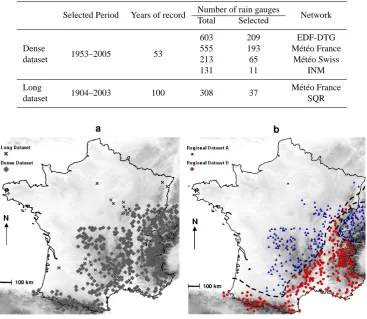
Table 2. Characteristics of the rainfall data sets.
Selected Period Years of record Number of rain gauges Network Total Selected
Dense
dataset 1953–2005 53
603 209 EDF-DTG
555 193 M´et´eo France
213 65 M´et´eo Swiss
131 11 INM
Long
dataset 1904–2003 100 308 37
M´et´eo France SQR
Fig. 1. (a) Rain gauges location. (b) Regional classification as a function of the “Season-at-risk”, i.e. the three consecutive months that
maximize the sum of the monthly rainfall maxima.
Both original datasets were first subject to a quality-check analysis, thus reducing the number of stations available for the model comparison. Only series with less than 10% of missing values per year were considered. Moreover, these series were further analysed to detect several anomalies: time shifts due to sensor replacement or station relocation, step changes or trends in rainfall intensity series.
The step change anomalies were studied by testing the stability over time of the residual of a multiple linear re-gression linking observations of the studied rain gauge with observations at the neighbouring rain gauges (Peterson and Easterling, 1994; Gottardi, 2009). Two statistics were com-bined in this test, based on the Alexandersson homogeneity test (Alexandersson, 1986) and of the sum of residuals with associated confidence intervals (Bois, 1976). Various tests are available for trend detection. In this study, we chose distribution-free tests because they do not require hypothe-ses on the data distribution (Hamed, 2009). According to Lang et al. (2006), two tests are commonly used to detect trends in non auto-correlated data series with unknown distri-bution: the Mann-Kendall test (Mann, 1945; Kendall, 1975) and Spearman’s rho test (Lehmann, 1975; Sneyers, 1990).
The Mann-Kendall test was selected since it is as powerful as Spearman’s rho test (Yue et al., 2002). 478 rain gauges from the dense dataset and 37 rain gauges from the long dataset were selected (Table 2) using this pre-processing. For both datasets, the most severe test has been the criterion on the percentage of missing value. For instance, concerning the long dataset, only 44 stations over 308 ( 14%) were selected. Among these remaining series, the trends detection led to discard 7 more stations. Figure 1a shows the location of the selected stations from the two datasets.
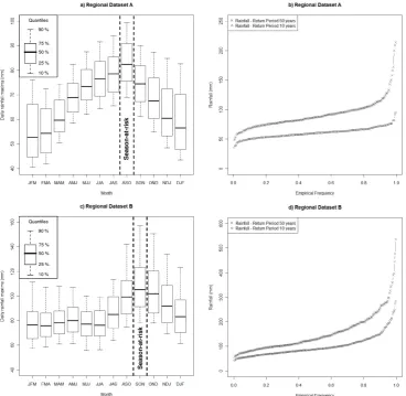
Fig. 2. Box plot of the three consecutive monthly rainfall maxima of regional dataset A (a) and regional dataset B (c). Empirical distribution
of rainfall quantile estimates associated with 10- and 50-year return periods for regional dataset A (b) and regional dataset B (d).
and October (regional dataset A) or between September and November (regional dataset B). Figure 2b and d show that the two regional data sets cover a large variability of rainfall intensities, from 40 to 170 mm (resp. 40 to 290 mm) for the empirical daily 10-year rainfall for dataset A (resp. B) and from 50 to 220 mm (resp. 70 to 520 mm) for the empirical daily 50-year rainfall for the dataset A (resp. B).
4 Comparison of probabilistic models
This section describes the strategy used to compare the prob-abilistic models, and defines several criteria to quantify the reliability and robustness of each model. Several statistical tests are reported in the literature to measure the goodness of fit: Pearson’s chi-square test (Plackett, 1983), Kolmogorov – Smirnov test (Kolmogorov, 1941; Smirnov, 1944), Ander-son – Darling Test (AnderAnder-son and Darling, 1952), Cramer-von-Mises criterion (Cramer, 1928; Darling, 1957), Shapiro-Wilk test (Shapiro and Shapiro-Wilk, 1965) and test of Lilliefors
This paper does not solely focus on goodness of fit, and instead attempts to evaluate the predictive performance of a model using independent validation data (i.e. not used to calibrate the model). Moreover, focus is on the tail of the distribution, i.e. the performance of the model in estimating the exceedance probability of large values. It is argued that the evaluation of goodness-of-fit is not sufficient to assess the ability of a model to predict the exceedance probability of future (unobserved) values. Consequently, we propose an alternative approach based on specific criteria computed on an extensive dataset.
A probabilistic model of extreme rainfall should be both reliable and robust. A reliable model assigns the “correct” exceedance probability to high values. In practice, this prop-erty can only be evaluated with respect to observed data. Consequently, it is useful to consider both long series and dense data sets in order to increase the sample of observed extreme values. On the other hand, a robust probabilistic model yields similar estimates when a slight perturbation of data is introduced. This property is very important, espe-cially in the extrapolation of extreme quantiles, in order to avoid an estimate being overly sensitive to sampling variabil-ity. Robustness is easier to quantify than reliability but an analysis solely based on the former is not sufficient because robustness does not give any information about the ability of the model to describe or predict observations. In the absence of reliability diagnostics, a robust model is not necessarily preferable: a model can be robust but totally unreliable. In conclusion these properties are complementary: the reliabil-ity of the model should be evaluated first, and in a second step, the most robust model (amongst reliable ones) should be preferred. Specific criteria quantifying reliability and ro-bustness are proposed in the following sections.
4.1 Reliability criteria
As mentioned above, measuring the reliability of probabilis-tic estimations of high quantiles is not an easy task. We take cues from methods developed in the context of skill assess-ment of probabilistic forecasts, in particular, the reliability diagram (also called attribute diagram) (Wilks, 1995). This tool is used to assess the consistency of a probabilistic fore-cast of binary events. It plots the observed frequency against the forecast probability in order to evaluate their agreement. This diagram is widely used in forecasts analysis and com-parisons (e.g. see Bartholmes et al., 2009, for an application). Similarly, we propose a specific procedure to evaluate the agreement between the exceedance probabilities of ex-treme events provided by a probabilistic model and their ob-served frequencies. This tool, named FF criterion, is based on a split-sample procedure and was introduced by Garc¸on (1995). LetDbe a regional data set ofLstations of length
N,Diis the time series at sitei. The computation of the FF criterion can be divided into the following steps:
1. Each Di is split into two successive sub-samples of equal lengthN/2:x1i,...,xN/2i
andxN/2i +1,...,xNi
. 2. Two cdf F1i(x) and F2i(x) of the same probabilistic
model are fitted using each sub-sample.
3. Let mi1 = maxnx1i,...,xN/2i o and mi2 =
maxnxN/2i +1,...,xNio. Under the hypothesis of i.i.d. random variables the probability of non-exceedance of mi1 (resp. mi2) is computed with the cdf fitted to the second part F2i(x) (resp. the first part F1i(x)) as follows:
FF1i=P r
Mi≤mi1
=
h F2i
mi1
iN/2
(1a)
FF2i=P rMi≤mi2
=hF1imi2i
N/2
(1b)
2Lvalues of probabilities FF are therefore computed. With a perfect probabilistic model, the distribution of FF values should be a Kumaraswamy’s double bounded distribution of parametersNand 1; i.e.K[N,1](Kumaraswamy, 1980); see Appendix A. A pp-plot is used to check this feature: the closer the FF distribution to the 1:1 diagonal, the more re-liable the probabilistic model.
In practice, the theoretical distributionsF1i(x)andF2i(x)
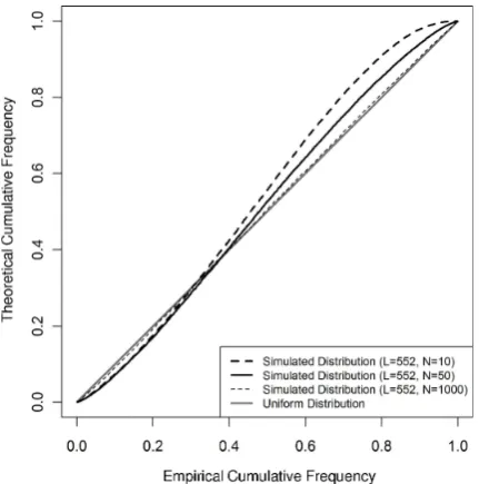
are replaced by their estimates based on samples of limited size, thus leading to departures from the 1:1 line. To quan-tify this, FF is calculated on 1000 random datasets of three different sample sizes, generated from an exponential pop-ulation. The size of the first sample is similar to that of the actual rainfall dataset (L=552,N=50), the second is smaller (L=552,N=10) and the third is bigger (L=552,
N=1000). Figure 3 shows the median of the simulated FF distributions for each dataset size. It appears that logically, the FF distribution plot moves closer to the 1:1 diagonal (the-oretical result) when the sample size increases. Because of the bias introduced by the limited sample size, the analysis of the reliability test is mainly qualitative and provides a way to compare concurrent probabilistic models.
The FF procedure is used to assess the ability of a proba-bilistic model to assign the “correct” probability to the high-est observed values that were not used for model fitting. With analogy with the split sample test, this kind of procedure can be named FF validation procedure. Note that the FF proce-dure solely focuses on the maximum observed value during the validation period: it is therefore primarily geared toward the assessment of reliability in the tail of the distribution.
Fig. 3. FF distribution provided by simulation with random
sam-ples extracted from an exponential distribution. Different curves represent three kinds of simulations with samples of different sizes.
same sub-sample can be used:
FF1i
∗
=P rMi≤mi1
=hF1imi1iN/2 (2a)
FF2i
∗
=P r
Mi≤mi2
=
h F2i
mi2
iN/2
(2b) This approach can be interesting in cases where the ob-served distribution of FF∗values is less variable than the the-oreticalK[N,1]distribution. Indeed, the latter distribution corresponds to what should be observed using the true distri-bution of data: it corresponds to a lower bound for the vari-ability of FF∗ values, solely resulting from sampling vari-ability. Consequently, a probabilistic model yielding FF∗ values less variable than the theoreticalK[N,1]distribution tends to “fit” extreme values, which is typical of over-parameterized models. With analogy to the FF validation procedure, this second approach can be named the FF cali-bration procedure.
In order to improve the comparison a robustness assess-ment is presented into the following paragraph.
4.2 Robustness criteria
The robustness is the ability of a method to yield close esti-mations when two different calibration periods are utilised. Robustness is quantified using several sub-samples of the whole long data series, in order to increase the reliability of the assessment. To analyse the results and compare the mod-els, two scores are computed: the SPANT criterion and the COVERTcriterion.
The SPANT criterion aims to evaluate the variability of extreme quantile estimation. This criterion can be defined as follows:
SPANT=
maxqˆT ,n=1,...,m −min
ˆ
qT ,n=1,...,m 1
m
Pm n=1qˆT,n
(3) whereqˆT,nis the model estimate for the return periodT and the sub-period n amongst mnon-overlapping sub-periods. The value of this score is greater or equal to 0, zero being the ideal score, occurring for a probabilistic model that is com-pletely unaffected by the sub-period used for calibration.
Moreover, it is reasonable to assert that a probabilistic model is more robust if the confidence intervals calculated for different sub-periods overlap well. Note that we are in-terested here in confidence interval overlap and not in their width. Indeed, for a given model and return period, two bootstrap confidence intervals (computed from two different sub-samples) could be narrow but totally disconnected. Such behavior is not in line with the robustness requirement. To quantify this property, a second criterion, named COVERTis derived. The analytical expression of this score is as follows: COVERT
= Qm
n=1P r max
ˆ
qT ,α/2,n=1,...,m ≤ ˆqT,n≤minqˆT ,1−α/2,n=1,...,m
(1−α)m
= Qm
n=1P r a≤ ˆqT,n≤b
(1−α)m (4)
where qˆT,α,n is the model estimate for the return level T with a confidence level αand computed on the sub-period
n(amongstmnon overlapping sub-periods). This is the nor-malized product of the probability densities of theqˆT quan-tile within thea−b interval, wherea is the highest value of the lower limit of the confidence intervals and b is the lowest value of the upper limit of the confidence intervals. This score therefore provides a quantitative value of the con-fidence interval overlap for each sub-period. The graphical explanation of the COVERTcriterion is shown in Fig. 4 for two sub-periods. This figure highlights that the optimum of the criterion is 1 (confidence intervals are identical), and the minimum value is 0 (confidence intervals are disconnected). 4.3 Comparaison methodology
Fig. 4. Schematic confidence intervals overlap criteria: COVERT. Xis the model estimate computed on the sub-period 1 with confidence interval[x−;x+]andY is the model estimate computed on the sub-period 2 with confidence interval[y−;y+].ais the highest value of the lower limit of confidence intervals andbis the lowest value of the upper limit of the confidence intervals. Three cases are shown: COVERT equal to 0 (null overlap), 0.5 (half overlap) and 1 (total overlap).
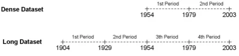
Fig. 5. Sub-period division of the two datasets.
years;L=478+2·37=552 stations). SPANTand COVERT criteria are computed for each station and for different return levels.
Alternative division schemes, yielding sub-periods with different length and/or random sub-periods (i.e. containing non-consecutive years) were also tested in order to check that the results were not influenced by climatic effects or by the relative length of calibration/validation periods. The sion scheme presented in Fig. 5 and these alternative divi-sion schemes led to similar results, so for a practical reason the latter results are not presented.
5 Results
This section presents the results of the model comparison. The GUM (resp. GEV) distribution performs closely to the EXP distribution (resp. GP) so for clarity’s sake the scores of GUM and GEV distributions appear only in the tables and not in the figures of this section.
5.1 Reliability
Starting with the reliability criteria, the FF calibration and validation criteria are calculated for the six models using the whole dataset. The results of these tests are presented through the pp-plot between the empirical and theoretical frequencies of the FF values (Fig. 6). According to these results the MGPWP performs as well as MEWP distribution
in validation but is the worst model in calibration. In par-ticular, the shape of the MGPWP pp-plot in calibration sug-gests that the observed FF values are less variable than the-oretically expected. As indicated in Sect. 4.1, this is typical of over-parameterised models. Fitting the shape parameter on each WP sub-sample, the MGPWP distribution tends to over-fit extreme values. However, and perhaps surprisingly, this does not result in a loss of predictive performance in val-idation. Overall, and based on both criteria (FF calibration and validation criteria) the MEWP distribution is the most reliable model given that its distribution is the closest to the 1:1 diagonal.
Compared to MEWP and MGPWP distributions, the EXP and GP distributions have a distinctly lower predictive per-formance in validation (Fig. 6, right panel): this highlights the value of weather-pattern sub-sampling in estimating ex-treme quantiles. Moreover, the EXP distribution performs better than the GP distribution, which may appear surprising. Nevertheless this result is due to high variability of estimated shape parameterξ for the GP distribution. This parameter is sometimes negative, corresponding to an upper-bounded dis-tribution. In such case, the FF validation criterion is equal to 1 if the maximum observed value in the validation period is greater than the upper bound (corresponding to an ”im-possible” observation according to the model). In the whole dataset and in all sub-periods (1104 stations·periods) 632 negative shape parameter were estimated (∼57%), yielding
[image:8.595.48.287.277.333.2]Fig. 6. pp-plot of FF scores in calibration and validation. Whole dataset is used to computed these distributions.
Table 3. Results of the reliability procedure for the six probabilistic models.
1
1−f(FF) f(FF)
A value exceeded one time over 10 according to:
Simulation EXP
is observed one time over
7 0.850
(M=552, N=50)
GUM 5 0.784
GEV 4 0.744
EXP 5 0.780
GPD 4 0.734
MEWP 7 0.866
MGPWP 8 0.869
A value exceeded one time over 20 according to:
Simulation EXP
is observed one time over
11 0.909 (M=552, N=50)
GUM 7 0.860
GEV 5 0.793
EXP 7 0.864
GPD 5 0.783
MEWP 11 0.913
MGPWP 15 0.931
A value exceeded one time over 100 according to:
Simulation EXP
is observed one time over
38 0.974 (M=552, N=50)
GUM 16 0.938
GEV 7 0.847
EXP 17 0.941
GPD 7 0.848
MEWP 34 0.970
MGPWP 32 0.969
Particular attention has to be paid to the highest frequency in the presented pp-plot. In this regard, the FF validation pro-cedure may be expressed for high quantiles as follows. For example, with the EXP distribution the empirical cumulative frequency of the 0.95 quantile of FFEXPis 0.86 (Fig. 7). This means that a value supposed to occur one time out of 20,
[image:9.595.154.442.315.622.2]Fig. 7. Close-up of the upper tail of the FF validation procedure.
The gray circles highlight the values shown in Table 3. Whole dataset is used to computed these distributions.
analysis. It shows that the MEWP and MGPWP distributions are less biased than the other distributions, with observed val-ues (resp. 7, 11 and 34 for the MEWP distribution and 8, 15, 32 for the MGPWP distribution) closer to both the theoret-ical values (resp. 10, 20 and 100) and the simulated values (resp. 7, 11 and 38) including the sampling effect (Fig. 3). 5.2 Robustness
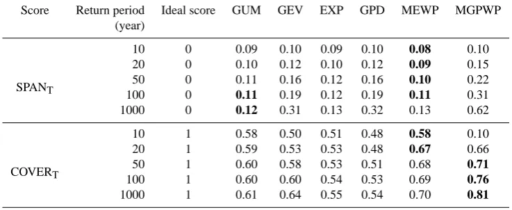
Figure 8 shows the empirical distributions of the two ro-bustness criteria (SPANT and COVERT) computed at the 20-years, 100-years and 1000-years return levels. The GP and the MGPWP distributions are the most sensitive to sampling variability, as the SPAN100 and SPAN1000 scores are markedly larger than with the other distributions. The SPAN20remains almost similar for all the considered mod-els (being MEWP the best one and MGPWP the worst one). Also in this case such a low level of robustness in these two models is due to high variations of the shape parameterξ in different sub-periods. Furthermore the MGPWP distribution drifts further away from the ideal SPANT than GP distribu-tions, especially for 1000-years return level. The other prob-abilistic models (EXP and MEWP distributions) yield similar and better SPAN100and SPAN1000scores.
In order to complete the robustness comparison, it is im-portant to pay attention to the confidence interval overlap. The MEWP and the MGPWP distribution have the empir-ical distribution of the COVER20 score closest to the ideal score. Instead in the case of the empirical distribution of the COVER100and COVER1000scores, the MGPWP
distri-bution performs better than the other ones. The good per-formance of MGPWP distribution in terms of COVERT cri-terion is a consequence of the width of its confidence in-tervals. Indeed, as the confidence intervals are wide, the probability to observe a good confidence interval overlap is higher. On the whole dataset, the MGPWP distribution at 100-years return level has in average an interval confidence width equal to ±0.76 of the central estimation. The EXP, GP and MEWP distributions have respectively interval con-fidence width equal to±0.17,±0.52 and±0.22 of the cen-tral estimation. The MEWP distribution yields satisfactory scores however its confidence interval size is appreciably moderate. The EXP and GP distributions are slightly less robust than the two distributions based on WP sub-sampling. Beside for these two models, the confidence intervals, com-puted on two different periods, appear totally disconnected for about 10% of the rain gauges (e.g. COVERTscore equal to 0).
A global robustness assessment may be summarized for the proposed criteria. Table 4 shows the mean SPANT and COVERT criteria at the 10-years, 20-years, 50-years, 100-years and 1000-100-years return levels for the six probabilistic models considered. According to the results shown in Fig. 8 and in Table 4, the MEWP distribution provides a good level of robustness, from moderate to high return levels, either for the variability of extreme quantile estimation (SPANT crite-rion) or for confidence interval overlap (COVERTcriteria).
6 Discussion and Conclusions
The aim of this paper was to assess a probabilistic model based on atmospheric circulation pattern by comparing it with standard probabilistic models derived from extreme value theory using an extensive data set. A specific method for the comparison of probabilistic models was introduced. Firstly, the reliability of the model to estimate extreme rain-fall quantiles was investigated. Secondly, the comparison examined the robustness of the extreme quantiles and their associated Bootstrap confidence intervals, based on various sub-samples of long data series (about 100 years). The use of long data series made it possible to compare the proba-bilistic models on extreme values. Seasonal variability of precipitation in France and in the surrounding area was taken into account.
Some interesting conclusions can be drawn. The results of the comparison clearly highlight the interest of a WP sub-sampling. In particularly the probabilistic models based on WP approach provide good predictive performance in vali-dation (FF valivali-dation criterion). This conclusion means to suggest that the number of parameter, a priori a negative fea-ture, does not affect the statistical qualities of the proposed probabilistic models based on WP.
Fig. 8. Empirical distribution of SPANTand COVERTcriteria at 20-years, 100-years and 1000-years return levels. Whole dataset is used to computed these distributions.
drop in robustness, overall for high (100-years and 1000-years) return levels. Therefore in operational application a regional analysis is recommended for robust estimation of shape parameter (Madsen et al., 1995; Martins et al., 2001; Ribatet et al., 2007; Pujol et al., 2008).
Table 4. Mean SPANTand COVERTcriteria (the numbers in bold highlight the best performance for each return period).
Score Return period Ideal score GUM GEV EXP GPD MEWP MGPWP (year)
SPANT
10 0 0.09 0.10 0.09 0.10 0.08 0.10
20 0 0.10 0.12 0.10 0.12 0.09 0.15
50 0 0.11 0.16 0.12 0.16 0.10 0.22
100 0 0.11 0.19 0.12 0.19 0.11 0.31
1000 0 0.12 0.31 0.13 0.32 0.13 0.62
COVERT
10 1 0.58 0.50 0.51 0.48 0.58 0.10
20 1 0.59 0.53 0.53 0.48 0.67 0.66
50 1 0.60 0.58 0.53 0.51 0.68 0.71
100 1 0.60 0.60 0.54 0.53 0.69 0.76
1000 1 0.61 0.64 0.55 0.54 0.70 0.81
of FF validation and COVERT criteria are observed, but on other hand this model presents a very low level of FF cali-bration and SPANTcriteria. This aspect strongly reduces its applicability in operational application for reasons of coher-ence and repeatability. However we plan to carry out a future investigation on the use of a GP distribution for the most se-vere WP, with a regional assessment of the shape parameter. In conclusion for daily data, the MEWP distribution presents a good level of reliability and robustness with re-spect to the proposed criteria. These conclusions may be dif-ferent with sub-daily data. It would be interesting to carry out the same kind of study based on hourly time-series even if data availability would then be an issue especially for the robustness of the results.
In the proposed comparison technique the spatial depen-dence between samples maxima was not taken into account. The spatial dependence could influence the results of the FF procedure, with a similar effect than the sampling effect pre-sented in Fig. 3. However, the spatial dependence should not change the global results for a comparison purpose since all models are applied to the same data, affected by the same spatial dependence. Also we plan to carry out a future in-vestigation on spatial distribution of computed scores and on correlation analyses between model performance and clima-tological features. The question of assessing the reliability (in addition to the robustness) of estimated uncertainties is also of interest. In our study the maximum likelihood method was used to fit models parameters. The uncertainties were not taken into account in the estimation of models parameters and so it could be potentially interesting to check if taking into account uncertainties (i.e. use a predictive distribution as models estimation, see Gelman et al., 1995) could improve reliability and robustness of models. Such developments are currently investigated within the French National research project named ExtraFlo 2009-2012 (EXTreme RAinfall and FLOod estimation: design values for extreme rainfall and floods. https://extraflo.cemagref.fr).
Appendix A
Reliability criterion FF Let:
– Da regional dataset ofMstations; – Di the time series at sitei;
– Nithe length of theDi time series; – mi the observed maximum ofDi; – Fˆi the probabilistic model fitted onDi.
The FF score at site i can be defined as follow:
FFi= ˆFi mi
If the estimation is perfectly reliableFˆi=Fi, then FFi∼ K
Ni,1
(Kumaraswamy’s double bounded distribution, Kumaraswamy, 1980), i.e. its cdf is P r FFi≤t=tNi
where 0≤t≤1. Proof:
P r FFi≤t =P r
ˆ
Fi mi≤t
. IfFˆi=Fi:
P rFFi≤t=P r
mi≤nFio −1
(t )
=P r
Dki≤nFio −1
(t )∀k=1,...,Ni
=
F
n Fio
−1
(t ) Ni
Acknowledgements. The authors would to acknowledge M´et´eo-France, M´et´eo-Swiss and Instituto Nacional de Meteorologa for the daily data sets. The referees are thanked for their helpful comments. F. Garavaglia would like to warmly acknowledge A. Mantovan for Fig. 4 and T. Mathevet for philosophical and hydrological discussions on the proposed criteria.
Edited by: R. Merz
References
Akaike, H.: A new look at the statistical model identification. IEEE Transactions on Automatic Control, 19, 6, 1974.
Alexandersson, H.: A homogeneity test applied to precipitation data, J. Climatol., 6, 661–675, 1986.
Anderson, T. W. and Darling, D. A.: Asymptotic theory of certain goodness-of-fit criteria based on stochastic processes, Annals of Mathematical Statistics., 23, 193–212, 1952.
Bardossy, A., Duckstein, L., and Bogardi, I.: Fuzzy rule-based clas-sification of atmospheric circulation patterns. International Jour-nal of Climatology., 15, 1087–1097, 1995.
Bartholmes, J. C., Thielen, J., Ramos, M. H., and Gentilini, S.: The european flood alert system EFAS – Part 2: Statistical skill as-sessment of probabilistic and deterministic operational forecasts, Hydrol. Earth Syst. Sci., 13, 141–153, doi:10.5194/hess-13-141-2009, 2009.
Bo´e, J. and Terray, L.: A weather type approach to analysing winter precipitation in France: twentieth century trends and influence of anthropogenic forcing, J. Climate, 21, 3118–3133, 2008. Bois, P.: Contrˆole de s´eries chronologiques corr´el´ees par ´etude du
cumul des r´esidus de la corr´elation, II Journ´ees Hydrologiques de l’ORSTOM, 89–1000, 1976.
Boughton, W. and Droop, O.: Continuous simulation for design flood estimation–a review. Environmental Modelling & Soft-ware., 18, 309–318, 2003.
CFGB: Design flood determination by the gradex method. 18th congress CIGB-ICOLD n2, nov., Bulletin du Comit´e Franc¸ais des Grands Barrages-FRCOLD News, 96, 1994.
Coles, S.: An introduction to statistical modeling of extreme values. Springer, London, 2001.
Coles, S., Perricchi, L., and Sisson, S.: A fully probabilistic ap-proach to extreme rainfall modelling, J. Hydrol., 273, 35–50, 2003.
Cramer, H.: On the composition of elementary errors, Skand. Ak-tuarietids., 11, 13–74 and 141–180, 1928.
Darling, D.A.: The Kolmogorov-Smirnov, Cramer-von Mises Tests. Annals of Mathematical Statistics, 28, 823–838, 1957.
Di Baldassarre, G., Laio, F., and Montanari, A.: Design flood es-timation using model selection criteria, Phys. Chem. Earth, 34, 606–611, 2009.
Djerboua, A. and Lang, M.: Scale parameter of maximal rainfall distribution: comparison of three sampling techniques. Revue des Sciences de l’Eau, 20, 111–125, 2007.
Efron, B.: Bootstrap methods: Another look at the jackknife. The Annals of Statistics?, 7, 1–26, 1979.
Garavaglia, F., Gailhard, J., Paquet, E., Lang, M., Garon, R., and Bernardara, P.: Introducing a rainfall compound distribution model based on weather patterns sub-sampling. Hydrol. Earth
Syst. Sci. Discuss., 7, 313–344, doi:10.5194/hessd-7-313-2010, 2010.
Garc¸on, R.: Oral communication. Statistical and Bayesian Methods in Hydrological Sciences. A joint UNESCO International Con-ference in honor of Jacques Bernier, September 11–13, Paris, 1995.
Gelman, A., Carlin, J. B., Stern, H. S., and Rubin, D. B.: Bayesian data analysis. Chapmann & Hall London, 1995.
Gottardi, F.: Estimation statistique et r´eanalyse des pr´ecipitations en montagne. PhD Thesis. Polytechnic Institute of Grenoble, p. 252, Grenoble, 2009.
Guillot P. and Duband D.: La m´ethode du gradex pour le calcul de la probabilit´e des crues `a partir des pluie, AISH Red Book, 84, 560, 1967.
Hamed, K.: Exact distribution of the Mann-Kendall trend test statis-tic for persistent data. J. Hydrol., 365, 86–94, 2009.
Karagiannidis, A., Karacostas, T., Maheras, P., and Makrogiannis, T.: Trends and seasonality of extreme precipitation characteris-tics related to mid-latitude cyclones in Europe, Adv. Geosci., 20, 39–43, doi:10.5194/adgeo-20-39-2009, 2009.
Kendall, M. G.: Rank correction methods. Griffin, London, 1975. Khamis, H. J.: The delta-corrected Kolmogorov-Smirnov test for
the two-parameter Weibull distribution, J. Appl. Stat., 24, 301– 301, 1997.
Kolmogorov, A. N.: Confidence limits for an unknown distribution function. Annals of Mathematical Statistics., 12, 461–463, 1941. Kumaraswamy, P.: A generalized probability density function for double-bounded random processes. Journal of Hydrology. 46, 79–88, 1980.
Laio, F.: Cramer-von Mises and Anderson-Darling goodness of fit tests for extreme value distribution with unknown parameters, Water Resour. Res., 40, W09308, doi:10.1029/2004WR003204, 2004.
Laio F., Di Baldassarre, G., and Montanari, A.: Model selec-tion techniques for the frequency analysis of hydrological ex-tremes. Water Resour. Res., 45, W07416, ISSN:0043-1397, doi:10.1029/2007WR006666, 2009.
Lang, M. and Desurosne, I.: Esquisse des risques de crues a l’´echelle euro-m´editerran´eenne: les premiers r´esultats du pro-gramme FRIEND-AHMY exploitant les mod`eles AGREGEE et TPG. 23emes Journ´ees de l’hydrauliques, Congr`es SHF Crues et Inondations, Nimes 14-15-16 September, 1994.
Lang, M., Ouarda, T. B. M. J., and Bob´ee, B.: Towards opera-tional guidelines for over-threshold modeling. J. Hydrol., 225, 103–117, 1999.
Lang M., Renard, B., Sauquet, E., Bois, P., Dupeyrat, A., Laurent, C., Mestre, O., Niel, H., Neppel, L., and Gailhard J.,: A national study on trends and variations of French floods and droughts, IAHS Publication, 308, 514–519, 2006.
Lehmann, E. L.: Nonparametrics, Statistical Methods Based on Racks. Holden-Day, Inc, California, 1975.
Leonard, M.; Metcalfe, A., and Lambert, M.: Frequency analysis of rainfall and streamflow extremes accounting for seasonal and climatic partitions, J. Hydrol., 348, 135–147, 2008.
Liao, M. and Shimokawa, T.: A new goodness-of-fit test for type-l extreme-value and 2-parameter Weibull distributions with esti-mated parameters, J. Stat. Comput. Sim., 64, 23–48, 1999. Lilliefors, H.: On the Kolmogorov-Smirnov test for normality with
1967.
Linderson, M.: Objective classification of atmospheric circulation over southern Scandinavia, Int. J. Climatol., 21, 155–169, 2001. Littmann, T.: An empirical classification of weather types in the Mediterranean Bassin and their interrelation with rainfall, Theor. Appl. Climatol., 66, 161–171, 2000.
Madsen, H., Rosbjerg, D., and Harremo¨es, P.: Application of the Bayesian approach in regional analysis of extreme rainfalls, Stochastic Environmental Research and Risk Assessment., 9, 77–88, 1995.
Mann, H. B.: Nonparametric tests against trend, Econometrica, 13, 245–259, 1945.
Martinez, C., Campins, J., Jans`a, A., and Genov´es, A.: Heavy rain events in the Western Mediterranean: an atmospheric pattern classification, Adv. Sci. Res., 2, 61–64, 2008.
Martins, E. A. and Stendinger, J. R.: Generalized maximum like-lihood Pareto-Poisson flood risk analysis for partial duration se-ries, Water Resour. Res., 37, 2559–2567, 2001.
M¨uller, M., Kaˇsspar, M., and Matschullat, J.: Heavy rains and extreme rainfall-runoff events in Central Europe from 1951 to 2002, Nat. Hazards Earth Syst. Sci., 9, 441–450, doi:10.5194/nhess-9-441-2009, 2009.
Nach´azel, K.: Estimation Theory in Hydrology and Water Systems (Developments in Water Science), Elsevier Science, 1993. Paquet, E., Gailhard, J., and Garc¸on, R.: Evolution de la m´ethode
du GRADEX: approche par type de temps et mod´elisation hy-drologique, La Houille Blanche., 5, 80–90, 2006.
Plackett, R. L.: Karl Pearson and the Chi-Squared Test, Int. Stat. Rev., 51, 59–72, 1983.
Peterson, T. and Easterling, D. R.: Creation of homogeneous com-posite climatological reference series, Int. J. Climatol., 14, 671– 679, 1994.
Pujol, N., Neppel, L., and Sabatier, R.: Regional tests for trend de-tection in maximum precipitation series in the French Mediter-ranean region, Journal des Sciences Hydrologiques, 52, 956– 973, 2008.
Ribatet, M., Sauquet, E., Gresillon, J., and Ouarda, T. B. M. J.: Usefulness of the Reversible Jump Markov Chain Monte Carlo Model in Regional Flood Frequency Analysis, Water Resour. Res., 43, W08403, doi:10.1029/2006WR005525, 2007. Rosbjerg, D. and Madsen, H.: Advanced approaches in PDS/POT
modelling of extreme hydrological events in Hydrology: Science & Practice for the 21th Century., 217–221, British Hydrological Society, London, 2004.
Schwarz, G.: Estimating the dimension of a model, Ann. Stat., 6, 461–464, doi:10.1214/aos/1176344136, 1978.
Shapiro, S. and Wilk, M. B.: An analysis of variance test for nor-mality (complete samples), Biometrika, 52, 3 and 4, 591–611, 1965.
Smirnov, N. V.: Approximate laws of distribution of random vari-ables from empirical data. Uspehi Matem. Nauk., 10, 179–206, 1944.
Sneyers, R.: On the statistical analysis of series of observations. World Meteorological Organisation. Technical note 143, WMO 415, 1990.
Trigo, R. M. and DaCamara, C. C.: Circulation weather types and their influence on the precipitation regime in Portugal, Interna-tional Journal of Climatology, 20, 1559–1581, 2000.
Wilks, D. S.: Statistical Methods in the Atmospheric Sciences: An Introduction. Academic Press, 467 pp., 1995.
Yarnal, B., Comrie, A. C., Frakes, B., and Brown, D. P.: Develop-ments and prospects in synoptic climatology. Int. J. Climatol. 21, 1923–1950, 2001.
Yue, S., Pilon, P., and Cavadias, G.: Power of the Mann-Kendall and Spearman’s rho tests for detecting monotonic trends in hy-drological series. J. Hydrol., 259, 254–271, 2002.