www.hydrol-earth-syst-sci.net/16/937/2012/ doi:10.5194/hess-16-937-2012
© Author(s) 2012. CC Attribution 3.0 License.
Earth System
Sciences
Influence of infiltration and soil storage capacity on the skewness
of the annual maximum flood peaks in a theoretically derived
distribution
A. Gioia1, V. Iacobellis1, S. Manfreda2, and M. Fiorentino2
1Dipartimento di Ingegneria delle Acque e di Chimica, Politecnico di Bari, Bari, Italia
2Dipartimento di Ingegneria e Fisica dell’Ambiente, Universit`a degli Studi della Basilicata, Potenza, Italia
Correspondence to: A. Gioia ([email protected])
Received: 10 April 2011 – Published in Hydrol. Earth Syst. Sci. Discuss.: 14 June 2011 Revised: 31 December 2011 – Accepted: 2 January 2012 – Published: 22 March 2012
Abstract. Understanding the spatial variability of key pa-rameters of flood probability distributions represents a strat-egy to provide insights on hydrologic similarity and building probabilistic models able to reduce the uncertainty in flood prediction in ungauged basins. In this work, we exploited the theoretically derived distribution of floods model TCIF (Two Component Iacobellis and Fiorentino model; Gioia et al., 2008), based on two different threshold mechanisms as-sociated to ordinary and extraordinary events. The model is based on the hypotheses that ordinary floods are generally due to rainfall events exceeding a constant infiltration rate in a small source area, while the so-called outlier events respon-sible for the high skewness of flood distributions are trig-gered when severe rainfalls exceed a storage threshold over a large portion of the basin. Within this scheme, a sensitivity analysis was performed with respect to climatic and geomor-phologic parameters in order to analyze the effects on the skewness coefficient and provide insights in catchment clas-sification and process conceptualization. The analysis was conducted to investigate the influence on flood distribution of physical factors such as rainfall intensity, basin area, and particular focus on soil behavior.
1 Introduction
The understanding of processes control on the shape of the flood frequency distribution is essential to extrapolate reli-able at-site predictions to large return periods and to de-fine meaningful similarity indicators between catchments for flood frequency estimation in ungauged catchments (Merz
and Bloschl, 2009). These physical interconnections may be explored using an upward approach (or model based), where a stochastic rainfall model is coupled with a runoff model using derived distributions (Eagelson, 1972; Raines and Valdes, 1993; Gottschalk and Weingartner, 1998; Fiorentino and Iacobellis, 2001; De Michele and Salvadori, 2002; Franchini et al., 2005; Bocchiola and Rosso, 2009) or Monte Carlo simulations (e.g. Beven, 1987; Loukas, 2002; Blazkova and Beven, 2002; Fiorentino et al., 2007).
The literature proposes several schemes and procedures for the theoretical derivation of flood probability distribu-tions. Most of the derived distributions developed so far are based on a single runoff generation scheme, but this may rep-resent a limitation in the description of runoff production. Moreover, it is not always clear how well a single component describes the complex dynamics of flood formation within the river basin. In this context, the presence of different runoff generation processes, such as the saturation excess and the infiltration excess, under different climatic conditions and the dynamics which control the transition between the two schemes, may provide interesting insights useful to find sim-ilarities and differences among river basins and among their processes for classification and regionalization. Sivapalan et al. (1990) accounted for the effect of different mechanisms of runoff generation (infiltration excess and saturation excess), while Iacobellis and Fiorentino (2000) introduced the partial contributing area as a random variable and considered only one runoff threshold associated to infiltration excess in arid basins or to saturation excess in humid basins.
(e.g. McGrath et al., 2007). Kusumastuti et al. (2007) focused on catchment storage and derived the flood fre-quency distributions by Monte Carlo simulations, using a non-linear conceptual rainfall-runoff model. Struthers and Sivapalan (2007) illustrate the impact of heterogeneity asso-ciated with threshold nonlinearities in the storage-discharge relationship associated with the rainfall-runoff process upon flood frequency behaviour. They introduced two storage thresholds, namely a field capacity storage and a catchment storage capacity, that identify two different flood frequency “regions”. The return period associated with the transition between these regions is directly related to the frequency of threshold exceedance.
Following this line of investigation, this paper describes the effects of different runoff production mechanisms on the generation of ordinary and extraordinary flood events, ex-ploiting the TCIF flood frequency distribution (Gioia et al., 2008). The study analyses the effects of climatic and ge-omorphologic parameters, with particular focus on soil be-haviour, on statistical flood moments and in particular on the skewness coefficient.
Some interesting results in this direction were already ob-tained by Iacobellis et al. (2002) exploiting the theoretical model proposed by Iacobellis and Fiorentino (2000). In par-ticular, they explored the spatial variability of the coefficient of variation of annual maximum floods. They derived a the-oretical dependence between the coefficient of variation (Cv) and the abstraction characteristics at the basin scale, the basin area and rainfall parameters. Their findings highlighted that
Cvfollows scaling relationships with basin area, with distinct behavior dependent on the dominant runoff mechanism. In particular, Cv decreases with area when the infiltration ex-cess mechanism dominates, whileCvincreases with area in humid and vegetated basins where saturation excess runoff takes place.
On the other hand, the skewness coefficient (Cs) can vary vastly in catchments, which apparently exhibit similar flood behaviour (Matalas et al., 1975). This may be due to the interaction of temporal varying observation periods and cli-mate fluctuations, single extreme events and observation er-rors (Merz and Bloschl, 2009). According to McCuen and Smith (2008), the flood skew estimation involves rainfall skew and watershed and channel storage. In their scheme, rainfall skew represents an upper bound on the population of runoff skew and flood skew decreases from the rainfall skew for the same location as storage increases.
In any case, the spatial variability of Cs plays a crucial role in the hierarchical approach for regional flood frequency analysis (Fiorentino et al., 1987) and is recognized as one of the main factors influencing the estimation of upper quantiles of annual peak flows (e.g. Strupczewski et al., 2011). Indi-cations on the physical controls on this specific parameter is essential for a reliable evaluation of the upper quantiles and for extrapolating at-site statistics to large return periods.
The paper is structured as follows. Section 2 briefly sum-marizes the main features of the TCIF model. In Sect. 3 the organization and main focus of the sensitivity analysis are explained. In Sect. 4 results of the sensitivity analysis are shown and commented. Section 5 reports conclusions and perspectives of this research.
2 Theoretically derived flood frequency distribution (TCIF model)
The TCIF distribution was derived by Gioia et al. (2008) under the hypothesis that in natural basins different mech-anisms of runoff generation may coexist, being in turn re-sponsible of the peak flow, depending on the characteristics of the rainfall event and on the antecedent moisture condi-tions. Thus, two components arise characterized by:
– L-type (frequent) response, occurring when rainfall in-tensity (ia,τ) exceeds a lower threshold fa,L, and re-sponsible of ordinary floods likely produced by a rel-atively small portion of the basinaL; the L-type (fre-quent) peak unit runoff is:ua,L=ξ(ia,τ−fa,L). – H-type (rare) response, occurring when rainfall
inten-sity exceeds a higher thresholdfa,H, and providing ex-traordinary floods mostly characterized by larger con-tributing areasaH; the H-type (rare) peak unit runoff is:
ua,H=ξ(ia,τ−fa,H).
Other assumptions of the TCIF distribution model are that rainfall and infiltration, averaged in space and time, scale with the contributing area with the following relationships:
E
ia,τ = I1a−ε = EiA,τ(a/A)−ε (1) fa,L = fA,L(aL/A)−εL (2)
fa,H = fA,H (aH/A)−εH. (3) The rainfall intensity is considered Weibull distributed (with shape parameterk) and the contributing areasaLandaHhave a continuous part, Gamma distributed, and a spike of discrete probability fora=Atotal basin area. These distributions are characterized by a parameterβwhich depends on the coeffi-cient of variation and is assumed constant. Other parameters areαL=rLA/βandαH=rHA/βwhich depend on the mean value, once theβ value is fixed, being the mean value rep-resented by the dimensionless parametersrL=E[aL]/Aand
rH=E[aH]/AwithrH≥rL.
Assuming that L-type and H-type events are independent and that both rates of occurrence are Poisson distributed, the overall process of exceedances is also a Poisson process, and the following relationships hold:
3H = 3pexp
−
fA,kH
EhikA,τi
and
3q = 3L +3H = 3pexp
−
fA,kL
EhikA,τi
. (5)
3Land3Hare the mean annual number of independent flood events for the L-type and the H-type events.
In compound Poisson processes, if the base process of rainfall intensity follows the exponential distribution, then the annual maximum rainfall intensity is Gumbel distributed. The exponential distribution corresponds to a Weibull distri-bution withk= 1. Then, in this case, we may write:
EhiA,τk i = E
iA,τ = IA =I1A−ε (6) withI1the rainfall intensity per unit contributing area andεa scaling coefficient dependent on the slope of the areal rainfall IDF (intensity duration frequency) curves.
The general expression of the cumulative probability distribution of the annual maximum flood peak and its probability density function are reported in Iacobellis et al. (2011). In the particular case of rainfall intensity expo-nentially distributed, the cumulative probability distribution, CDFQp(qp), of the annual maximum flood peakqp=Q+qo, withqo the base flow, and its probability density function become:
CDFQp qp
=
exp
−3L
A
Z
0
g (aL)exp
− qp −qo
/(ξ aL)
E
iaL,τ
!#
daL
)
· exp
−3H
A
Z
0
g (aH)exp − qp −qo
/(ξ aH)
E
iaH,τ
!
daH
(7)
PDFQp qp
=CDFQp qp
3L
A Z 0
g (aL)
1
(ξ aL) EiaL,τ
exp −
qp −qo
/(ξ aL)
EiaL,τ
!
daL
)
+3H
A Z 0
g (aH)
1
(ξ aH) EiaH,τ
exp − qp −qo
/(ξ aH)
E
iaH,τ
!
daH
)#
. (8)
E[iaL,τ]andE[iaH,τ] are, respectively, the average rainfall
intensity with respect to contributing areasaL andaH,ξ is a constant routing factor,g(aL)andg(aH)are, respectively, the probability density functions of the L-type and H-type contributing areas.
3 Methodology and organization of the sensitivity analysis
In Gioia et al. (2008) and Iacobellis et al. (2011), particu-lar attention was paid to the dynamics of runoff source ar-eas by revealing the scaling behaviour of the runoff thresh-olds (fA,LandfA,H). In particular, investigating the ent mechanisms of runoff production that coexist in differ-ent climates, they found that the scaling behaviour of the H-type (rare events) runoff threshold corresponds to a storage threshold associated to a mechanism of infiltration excess. This kind of response arises when an intense and persistent rainfall of significant areal extension exceeds a water storage capacity over large and more or less vegetated hillslopes. On the other hand, the L-type (frequent events) runoff threshold corresponds to a constant (and low) infiltration rate associ-ated to a saturation excess mechanism.
In order to keep trace of the different role of infiltration rate and soil storage capacity and soil storage capacity in the proposed sensitivity analysis, we characterize the two runoff thresholds considering the lower thresholdfA,Las associated to the spatial average of a constant soil infiltration rate in saturated conditions,φ,
fA,L ∼= φ. (9)
Then, we consider the soil water storage capacity averaged in space and over the basin lag-time, which scales with basin area as:
WA = W1A−0.5; (10)
the higher runoff threshold can be evaluated as:
fA,H ∼= φ +WA. (11)
When rainfall exceeds the lower threshold, a small source areaaLcorresponding to the first (L-type) component is ac-tivated with mean annual number of exceedances equal to
3q=3H+3L(see Eq. 5). The exceedances of the second runoff threshold characterize the activation of a larger source area aH corresponding to the second (H-type) component with mean annual number of exceedances equal to3H(see Eq. 4).
Table 1. Frequency of rainfall exceedance over different thresholdsφandWA.
Soil storage capacity (WA) P (i > φ)
P (i > WA+φ) Low Medium High
Constant
infiltration
rate
(
φ
)
frequent frequent frequent
Low
frequent occasional rare
occasional occasional occasional
Medium
occasional rare very rare
rare rare rare
High
rare very rare extremely rare
Table 2. Expected basin behaviour, in terms of presence and weight of the two components, based on a broad classification of the different thresholdsφandWA.
Soil storage capacity (WA)
CDF type Low Medium High
Constant
infiltration
rate
(
φ
)
Low 1 component 2 components 2 components
(1st may be not relevant) (1st may be not relevant)
Medium 1 component 2 components 2 components (both are relevant) (2nd may be not observed)
High 1 component 2 components 2 components
(2nd may be not observed) (2nd may be not observed)
the constant infiltration rate at saturationφ, the probability of rainfall to exceed the first runoff threshold is high; for in-creasingφvalues, the number of rainfall events that exceeds the first runoff threshold becomes occasional for mediumφ
and rare for high φ. Then, if the storage capacityWA as-sumes values belonging to the lower class, the occurrence of exceedances of the second runoff threshold is frequent, occasional and rare, as it is in the range of variation of the constant infiltration rateφ (first column in Table 1); for a medium value ofφ, the occurrence of the exceedances is oc-casional, rare, and very rare (second column in Table 1), and for highφ value it becomes rare, very rare, and extremely rare (third column in Table 1).
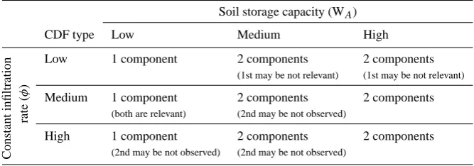
Following the above arguments, we report in Table 2 the expected behaviour of a basin regime in terms of presence and relevance of the two runoff components. For low values of the soil storage (WA), the two runoff thresholds are close (see Eqs. 9 and 11); then, it is possible to recognize only one component (L-type) of the theoretical model (first column of Table 2). When soil storage increases the second component
may become distinguishable; in particular for medium values of the soil storage, the first component may be not relevant to the right tail of the flood frequency curve if the constant infil-tration rateφis low (only the H-type component is present). On the other hand, ifφis high the second runoff threshold assumes very high values; then the second component may become not observable. Even for high values of soil storage, with increasing the values ofφ, the frequency of exceedances of the second runoff threshold will be so low that the second component may be not observable and not significant for re-turn periods of technical interest. It happens that only for medium values of bothφandWA, the two components are both relevant to the right tail of the flood frequency curve.
[image:4.595.130.464.325.442.2]Table 3. Mean annual number of events of the 2nd component (H-type response) based on different values of3Qand3H/3Q.
3H
3Q 3H/3Q
1/3 1/10 1/20 1/50 1/200 1/1000 High 20 6.667 2.000 1.000 0.400 0.100 0.020 Medium 10 3.333 1.000 0.500 0.200 0.050 0.010 Low 5 1.667 0.500 0.250 0.100 0.025 0.005
equal to the number of rainfall events that exceed the first thresholdφ, and the average annual number of flood events
3H exceeding also the second threshold WA+φ. Accord-ing to the variability of3q observed in Southern Italy (see Iacobellis et al., 2011), we considered values of 5, 10 and 20 flood events per year as representative of, respectively, low, medium and high frequency. For the occurrence of the second runoff threshold we considered six values obtained by adopting a fixed ratio between the mean annual number of occurrences3Hand3q (1/3, 1/10, 1/20, 1/50, 1/200 and 1/1000).
Under the hypothesis of rainfall intensity exponential dis-tributed, withk= 1, and replacing Eqs. (6) and (11) in Eq. (4) we obtain:
φ+WA IA
= −ln
3H
3p
. (12)
Replacing Eqs. (6) and (9) in Eq. (5), we obtain:
φ IA
= −ln
3
q
3p
; (13)
and combining Eqs. (12) and (13), we obtain:
WA IA
= −ln
3H
3q
. (14)
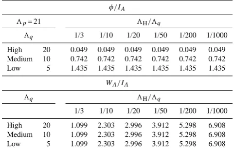
Following Eq. (14), the ratio 3H/3q depends only on WA/IA. Moreover, following Eqs. (12) and (13), for a fixed value of3p,3qdepends only on the ratioφ/IA, and3H de-pends only on the ratio (φ+WA)/IA. Therefore, for a fixed value of3p, of the ratio3H/3qand of3qit is possible to calculate the corresponding values ofφ/IA andWA/IA. In Table 4 we report the values of the dimensionless ratiosφ/IA obtained by means of Eq. (13), for3p= 21 and different val-ues of3q and3H. Table 4 reports also the values of the dimensionless ratio WA/IA obtained by means of Eq. (14) for different values of3qand3H. In both cases the corre-sponding values of3Hare those reported in Table 3 for the same3q-row and3H/3q-column. For known values ofφIA andWA/IA,φandWAcan be obtained according to values ofI1,Aandε, which, following Eq. (6), provideIA. Other parameters affecting the TCIF cumulative distribution func-tion in Eq. (7) are the ratios of the average contributing areas
[image:5.595.308.549.100.254.2]rLandrHduring a L-type and H-type event, respectively.
Table 4. Values of dimensionless ratiosφ/IA (for3p= 21) and WA/IA, based on different values of3qand3H/3q.
φ/IA
3p= 21 3H/3q
3q 1/3 1/10 1/20 1/50 1/200 1/1000
High 20 0.049 0.049 0.049 0.049 0.049 0.049 Medium 10 0.742 0.742 0.742 0.742 0.742 0.742 Low 5 1.435 1.435 1.435 1.435 1.435 1.435
WA/IA
3q 3H/3q
1/3 1/10 1/20 1/50 1/200 1/1000 High 20 1.099 2.303 2.996 3.912 5.298 6.908 Medium 10 1.099 2.303 2.996 3.912 5.298 6.908 Low 5 1.099 2.303 2.996 3.912 5.298 6.908
The sensitivity analysis was performed by numerically evaluating the TCIF cumulative distribution function and its probability density function, PDFQp(qp), for different sets of parameters3p,I1,ε,A,rL,rH,3H/3qand3q, and keeping constant the values of the following other parameters:
– the routing factorξ assumed equal to 0.7, as in Iacobel-lis and Fiorentino (2000);
– the shape parameterβof the gamma distribution of the contributing areas assumed equal to 4, as in Iacobellis and Fiorentino (2000);
– the exponents εL and εH of the power law relation-ship between infiltration losses and contributing area assumed, respectively, equal to 0 and 0.5, as reported in Gioia et al. (2008). The skewness coefficient of the distribution was evaluated by numerically solving the equation:
Cs =
R+∞
−∞ qp −µ qp
3
PDFQp qp
dqp
hR+∞
−∞ qp −µ qp
2
PDFQp qp
dqp
i3/2
;
with µ qp =
Z +∞
−∞
qpPDFQp qp
dqp. (15)
In order to provide a structured analysis of the influence of physical factors such as soil infiltration rate at saturation and soil storage capacity on the TCIF distribution and its skew-ness, the values of3Hand3qwere selected on the basis of Table 3, hence, for fixed values of the ratio3H/3q. Then, in order to analyze the roles ofφandWA, we used the ratios φ/IAandWA/IAshown in Table 4.
Table 5. Mean and standard deviation of skewness forrL= 0.1,rH= 0.3;Aranges from 10 to 500 km2andI1ranges from 10 to 50 mm h−1.
Mean of skewness
WA/IA= 1.098 WA/IA= 2.302 WA/IA= 2.996 WA/IA= 3.912 WA/IA= 5.298 WA/IA= 6.908
φ/IA= 0.049 1.858 2.252 2.260 2.053 1.743 1.612
φ/IA= 0.742 1.999 2.324 2.248 1.995 1.714 1.608
φ/IA= 1.435 2.225 2.452 2.308 2.039 1.792 1.707
Standard deviation of skewness
WA/IA= 1.098 WA/IA= 2.302 WA/IA= 2.996 WA/IA= 3.912 WA/IA= 5.298 WA/IA= 6.908
φ/IA= 0.049 0.025 0.066 0.082 0.077 0.049 0.034
φ/IA= 0.742 0.017 0.038 0.038 0.021 0.006 0.016
φ/IA= 1.435 0.011 0.018 0.010 0.009 0.028 0.035
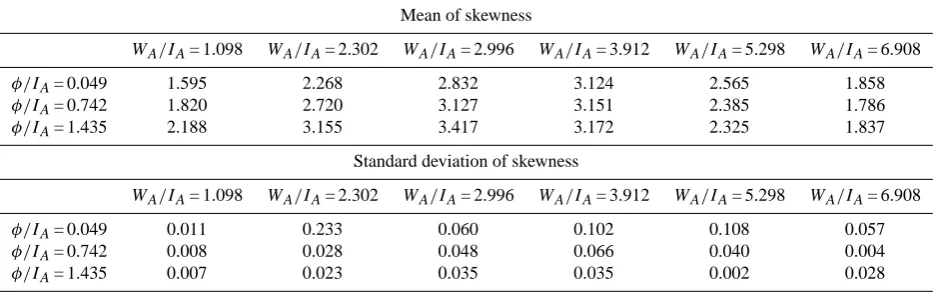
Table 6. Mean and standard deviation of skewness forrL= 0.1,rH= 0.6;Aranges from 10 to 500 km2andI1ranges from 10 to 50 mm h−1.
Mean of skewness
WA/IA= 1.098 WA/IA= 2.302 WA/IA= 2.996 WA/IA= 3.912 WA/IA= 5.298 WA/IA= 6.908
φ/IA= 0.049 1.595 2.268 2.832 3.124 2.565 1.858
φ/IA= 0.742 1.820 2.720 3.127 3.151 2.385 1.786
φ/IA= 1.435 2.188 3.155 3.417 3.172 2.325 1.837
Standard deviation of skewness
WA/IA= 1.098 WA/IA= 2.302 WA/IA= 2.996 WA/IA= 3.912 WA/IA= 5.298 WA/IA= 6.908
φ/IA= 0.049 0.011 0.233 0.060 0.102 0.108 0.057
φ/IA= 0.742 0.008 0.028 0.048 0.066 0.040 0.004
φ/IA= 1.435 0.007 0.023 0.035 0.035 0.002 0.028
on a set of river basins in Southern Italy investigated in pre-vious studies (Gioia et al., 2008; Fiorentino et al., 2011; Ia-cobellis et al., 2011). In particular, the mean annual num-ber of rainfall events3pranges from 21 to 75 (event/year), the rainfall intensity per unit of contributing areaI1 varies from 10 to 50 mm h−1, the basin areaAranges from 10 to 500 km2; the rainfall scaling coefficient ε varies from 0.3 to 0.4; and the ratios of mean contributing arearL andrH range from 0 to 1 with rH>=rL. We first report results for the entire observed variability of rL, rH, basin area A
and rainfall intensityI1and for the fixed values3p= 21 and ε= 0.3. Significant results obtained for different values of
3p andε are also discussed, provided that changing these last two parameters does not affect qualitatively the results and their implications on the paper focus, which is the un-derstanding of the role of soil infiltration rate at saturation and soil storage capacity on the presence of two runoff com-ponents and on the flood distribution skewness. We did not introduce any change of parametersξ andβ because in all the applications performed on real cases in previous studies
they did not show any variability. In the present application, the base flowqois set to zero, because in the TCIF model, qo is added as a constant factor to the peak flow and hence does not affect the peak flow distribution. Finally, the anal-ysis does not account for changes in the shape parameterk
of the rainfall pdf (i.e. of rainfall skewness), which is left to further research.
4 Results and discussion
Results of the sensitivity analysis are described in the present section with particular emphasis on the skewness coefficient of the theoretical distributions. Results are reported in the form of growth curve probability plots and summarized in tabular form (see Tables 5–9).
According to the index flood method (NERC, 1975), the growth curve represents, by definition, the cdf of the growth factor
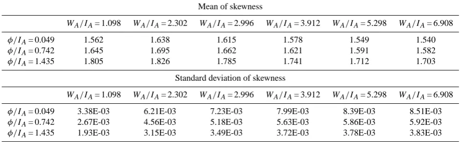
[image:6.595.64.533.292.438.2]Table 7. Mean and standard deviation of skewness forrL= 0.3,rH= 0.6;Aranges from 10 to 500 km2andI1ranges from 10 to 50 mm h−1.
Mean of skewness
WA/IA= 1.098 WA/IA= 2.302 WA/IA= 2.996 WA/IA= 3.912 WA/IA= 5.298 WA/IA= 6.908
φ/IA= 0.049 1.562 1.638 1.615 1.578 1.549 1.540
φ/IA= 0.742 1.645 1.695 1.662 1.621 1.591 1.582
φ/IA= 1.435 1.805 1.826 1.785 1.741 1.712 1.703
Standard deviation of skewness
WA/IA= 1.098 WA/IA= 2.302 WA/IA= 2.996 WA/IA= 3.912 WA/IA= 5.298 WA/IA= 6.908
φ/IA= 0.049 3.38E-03 6.21E-03 7.23E-03 7.99E-03 8.39E-03 8.51E-03
φ/IA= 0.742 2.67E-03 4.56E-03 5.18E-03 5.63E-03 5.86E-03 5.92E-03
φ/IA= 1.435 1.93E-03 3.15E-03 3.49E-03 3.72E-03 3.78E-03 3.83E-03
1 2 3 4 5 6
101 102 103
Kx
T
1 2 3 4 5
101 102 103
Kx
T
1 2 3 4 5 6
101 102 103
Kx
T
1 2 3 4 5 6
101 102 103
Kx
T
1 A A
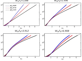
Fig. 1. Growth curves obtained forrL= 0.1,rH= 0.3, and different values ofφ/IA(as in the legend),I1(10, 50 mm h−1),A(10, 50, 100, 200, 500 km2),WA/IA(in subplots).
whose distribution is independent from the expected value, being obviously E[Kx]= 1. The growth curve depends on the coefficient of variation and on the skewness of the distri-bution. The TCIF arises as a distribution of annual maximum of a Poisson compound process, just as many other distribu-tions of extreme values (e.g. GEV, TCEV). The coefficient of variation of such distributions mainly depends on the mean annual number of flood events3q, and the TCIF distribution does not make an exception as it was confirmed by numer-ical investigation. Thus, the representation of TCIF growth curves characterized by the same value of3q and different values of the other parameters allows the identification of shape changes on the growth curve, with direct reference to
[image:7.595.127.470.265.513.2]Table 8. Mean and standard deviation of skewness forrL= 0.3,rH= 0.9;Aranges from 10 to 500 km2andI1ranges from 10 to 50 mm h−1.
Mean of skewness
WA/IA= 1.098 WA/IA= 2.302 WA/IA= 2.996 WA/IA= 3.912 WA/IA= 5.298 WA/IA= 6.908
φ/IA= 0.049 1.472 1.692 1.696 1.638 1.570 1.544
φ/IA= 0.742 1.585 1.779 1.755 1.680 1.610 1.586
φ/IA= 1.435 1.784 1.935 1.885 1.799 1.730 1.707
Standard deviation of skewness
WA/IA= 1.098 WA/IA= 2.302 WA/IA= 2.996 WA/IA= 3.912 WA/IA= 5.298 WA/IA= 6.908
φ/IA= 0.049 2.33E-03 5.16E-03 6.49E-03 7.62E-03 8.29E-03 8.51E-03
φ/IA= 0.742 1.85E-03 3.90E-03 4.76E-03 5.44E-03 5.80E-03 5.91E-03
φ/IA= 1.435 1.36E-03 2.80E-03 3.31E-03 3.64E-03 3.78E-03 3.83E-03
1 2 3 4 5 6
101 102 103
Kx
T
1 A A
2 4 6 8
101 102 103
Kx
T
1 A A
1 2 3 4 5
101 102 103
Kx
T
1 A A
2 4 6 8
101 102 103
Kx
T
[image:8.595.133.470.271.523.2]1 A A
Fig. 2. Growth curves obtained forrL= 0.1,rH= 0.9, and different values ofφ/IA(as in the legend),I1(10, 50 mm h−1),A(10, 50, 100, 200, 500 km2),WA/IA(in subplots).
from the lower part of Table 4, first, third, fourth and sixth columns). We grouped by colour all cdfs with the same value of φ/IA (i.e. with the same3q and Coefficient of Varia-tion): in blueφ/IA= 0.049 (3q= 20), in redφ/IA= 0.742 (3q= 10), in blackφ/IA= 1.435 (3q= 5). In each subplot, the three groups of cdfs differ in both the scale and the shape factor. As a first important evidence in Figs. 1 and 2, we observe that the TCIF cdfs obtained using different values of basin areaAand rainfall intensityI1, and keeping con-stant the ratiosWA/IA andφ/IA, practically collapse into one curve. Thus, in Tables 5–9, for a set of couples ofrL
andrH values, (rL= 0.1 andrH= 0.3 in Table 5,rL= 0.1 and
Table 9. Mean and standard deviation of skewness forrL= 0.1,rH= 0.9;Aranges from 10 to 500 km2andI1ranges from 10 to 50 mm h−1.
Mean of skewness
WA/IA= 1.098 WA/IA= 2.302 WA/IA= 2.996 WA/IA= 3.912 WA/IA= 5.298 WA/IA= 6.908
φ/IA= 0.049 1.400 2.130 2.729 3.346 3.096 2.097
φ/IA= 0.742 1.611 2.585 3.185 3.565 2.888 1.962
φ/IA= 1.435 1.994 3.144 3.662 3.723 2.761 1.966
Standard deviation of skewness
WA/IA= 1.098 WA/IA= 2.302 WA/IA= 2.996 WA/IA= 3.912 WA/IA= 5.298 WA/IA= 6.908
φ/IA= 0.049 7.89E-03 2.37E-02 4.30E-02 8.60E-02 1.29E-01 7.67E-02
φ/IA= 0.742 6.01E-03 2.03E-02 3.78E-02 6.70E-02 6.33E-02 1.10E-02
φ/IA= 1.435 4.78E-03 1.82E-02 3.21E-02 4.53E-02 1.90E-02 2.11E-02
rL = 0.3 rH = 0.6 rL = 0.1 rH = 0.3
1 2 3 4
101 102 103
Kx
T
1 2 3 4
101 102 103
Kx
T
rL = 0.3 rH = 0.9
1 2 3 4
101 102 103
Kx
T
1 A rL = 0.1 rH = 0.9
1 2 3 4
101 102 103
Kx
T
1 A
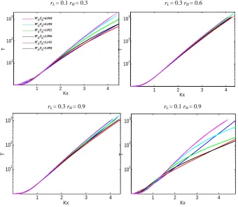
Fig. 3. Growth curves obtained for a constant value ofφIA(0.742), and varyingWA/IA(as in the legend),I1(10, 50 mm h−1),A(10, 50, 100, 200, 500 km2),rLandrH(in subplots).
of basin area and rainfall intensity. The results show a stan-dard deviation always significantly lower than the average coefficient of skewness.
Observing more carefully results reported in Tables 5–9, one may appreciate the effects of model parameters on skew-ness coefficient. In Table 5, for rL= 0.1 and rH= 0.3, the mean coefficient of skewness ranges from 1.608 to a maxi-mum value of 2.452. In Table 6, forrL= 0.1, rH= 0.6, the
[image:9.595.128.469.265.561.2]rL = 0.1 rH = 0.3
1 2 3 4 5
101 102 103
Kx
T
A A
rL = 0.3 rH = 0.9 rL = 0.1 rH = 0.9
rL = 0.3 rH = 0.6
1 2 3 4 5
101 102 103
Kx
T
1 2 3 4 5
101
102
103
Kx
T
1 2 3 4 5
101 102 103
Kx
T
[image:10.595.131.468.61.384.2]A A
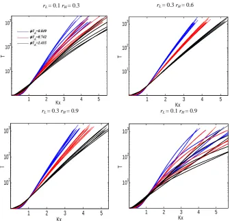
Fig. 4. Growth curves obtained varyingφIA(as in the legend),WA/IA(as in Table 4),I1(10, 50 mm h−1),A(10, 50, 100, 200, 500 km2),
rLandrH(in subplots).
which is also the highest value observed over all the parame-ter sets. In general, comparing results of Tables 5–9, a strong relationship between skewness andφ can be observed. In fact, the minimum value of the coefficient of skewness is al-ways observed for low values ofφandWA that may be ei-ther low or high. On the oei-ther hand, a peak of skewness is always observed for medium values ofWAand for medium or high values ofφ. In other words, the coefficient of skew-ness shows maximum values for medium-high values of the soil infiltration rate at saturation and medium values of soil storage capacity. It is important to highlight the consistency of these results with contents of Table 2. In fact, the skewness is high when both components of flood distribution affect the distribution of extreme flood events because they are not too low in order to be relevant and are not too rare in order to be observed. The skewness is low when only one component is relevant because either one of the two thresholds is low or the second threshold is high and exceedances are too rare to be observed.
In order to better understand the comparison among the different curves, accounting for both the scale factor and the shape factor effects, in Fig. 3 are reported different growth curves for four couples ofrLandrHwith a different
organization with respect to those reported in Figs. 1 and 2. In this case, each subplot reports different TCIF cdfs that have a fixed ratioφ/IA and variable values ofWA/IA (only curves for the medium value ofφ/IA are shown),I1andA. Obviously, even in these subplots the cdfs obtained for differ-ent values ofI1andAcollapse into one curve, but the colour code is used in order to identify different values ofWA/IA. Sinceφ/IAis fixed, in each of these subplots all curves have the same scale factor. Then the differences shown by the dif-ferent values ofWA/IAare all due to the curve shape factor, i.e. the coefficient of skewness. By comparing the four sub-plots of Fig. 3, one could notice that the minimum skewness is provided by a higher value ofrL(0.3). On the other hand, the largest scatter is observed with a low value ofrL(0.1) and a highrH(0.9).
Table 10. Mean and standard deviation of skewness for different values ofrL=rH;Aranges from 10 to 500 km2andI1ranges from 10 to 50 mm h−1.
rL=rH= 0.05 rL=rH= 0.3
Mean of Standard deviation Mean of Standard deviation
skewness of skewness skewness of skewness
φ/IA= 0.049 1.597 4.39E-02 φ/IA= 0.049 1.538 8.70E-03 φ/IA= 0.742 1.631 3.92E-02 φ/IA= 0.742 1.580 6.01E-03 φ/IA= 1.435 1.743 3.26E-02 φ/IA= 1.435 1.701 3.90E-03
rL=rH= 0.1 rL=rH= 0.9
Mean of Standard deviation Mean of Standard deviation
skewness of skewness skewness of skewness
[image:11.595.49.294.117.474.2]φ/IA= 0.049 1.574 2.92E-02 φ/IA= 0.049 1.235 3.16E-05 φ/IA= 0.742 1.579 1.94E-02 φ/IA= 0.742 1.264 7.07E-05 φ/IA= 1.435 1.684 3.74E-02 φ/IA= 1.435 1.377 7.38E-05
Fig. 5. Growth curves obtained forrL=rH= 0.05 and varyingφ/IA (as in the legend),WA/IA (as in Table 4),I1(10, 50 mm h−1),A
(10, 50, 100, 200, 500 km2).
For the same values of3p= 21 andε= 0.3, we report in Table 10 four cases obtained with rL=rH= 0.05, 0.1, 0.3 and 0.9. As shown in Fig. 5, relative torL=rH= 0.05, all cdfs with the same value ofφ/IAand different values ofI1, Aand alsoWA/IA collapse into one group of curves, with a practically null scatter. Other values of rL=rH provide analogous behaviour. In this case the mean value and the standard deviation of the coefficients of skewness are eval-uated on a set of 60 cdfs obtained, for any value of φ/IA, by combining the ratiosWA/IA= 1.098, 2.302, 2.996, 3.912, 5.298, 6.908 (as in bottom part of Table 4) with the values of basin areaA= 10, 50, 100, 200, 500 km2and the rainfall intensitiesI1= 10, 50 mm h−1. Also in this case the stan-dard deviation is always significantly smaller than the aver-age skewness. Results in Table 10 show that the skewness
Cs max= 0.027*rH/(rL
2 ) + 1.60 R2 = 0.94
Cs max = 0.019*rH/(rL 2
) + 1.516 R2 = 0.92
0.0 0.5 1.0 1.5 2.0 2.5 3.0 3.5 4.0 4.5
0 20 40 60 80 100
rH/(rL 2
)
C
s
m
a
x
ε = 0.4 ε = 0.3
Λινεαρε (ε = 0.3)
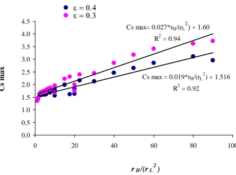
Fig. 6. Maximum skewness coefficient vs. rH/rL2, for 3p= 21,
ε= 0.3 (magenta) and3p= 21,ε= 0.4 (blue).
always grows with φ and higher skewness is obtained for lower values ofrL=rH. The minimum value of the skewness is 1.235 and is obtained for the highest value ofrL=rH= 0.9. This value, which is also the minimum value observed over the entire dataset of simulations, is not far from but signifi-cantly higher than the skeweness coefficient of a Gumbel dis-tribution which is equal to 1.13955. Analogous evaluations were performed considering different values of 3p andε, parameters that reflect, respectively, the rainfall coefficient of variation (3p) and the average rainfall scaling with area (ε, see Eq. 6). In particular for3p= 75 andε= 0.3,3p= 21 andε= 0.4, and3p= 40 andε= 0.4: in all cases the results confirm the behaviour displayed for3p= 21 andε= 0.3.
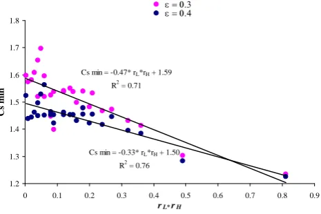
[image:11.595.312.543.298.469.2] [image:11.595.48.288.302.475.2]Cs min = -0.47* rL*rH + 1.59
R2 = 0.71
Cs min = -0.33* rL*rH + 1.50
R2 = 0.76
1.2 1.3 1.4 1.5 1.6 1.7 1.8
0 0.1 0.2 0.3 0.4 0.5 0.6 0.7 0.8 0.9
rL*rH
C
s
m
in
[image:12.595.52.285.64.219.2]ε = 0.3 ε = 0.4 Λινεαρε (ε = 0.3)
Fig. 7. Minimum skewness coefficient vs. rL·rH for3p= 21, ε= 0.3 (magenta) and3p= 21,ε= 0.4 (blue).
exists between the coefficient of skewness and the parameters
rLandrH, independently from the variability of all other pa-rameters. As we report in Fig. 6, the values of the maximum coefficient of skeweness, obtained for different values ofrL andrHby varying the other parameters, show a strong linear dependence on the ratio rH/rL2. On the other hand, Fig. 7 reports a dependence between the minimum coefficient of skewness and the productrH·rLobtained by varyingI1,A,
WA/IA andφ/IA. In Figs. 6 and 7 we also show results obtained for several other couples ofrL andrH reported in Table 11.
5 Conclusions
The sensitivity analysis performed over parameters of the TCIF distribution provides interesting insights on the con-trol that some physically-based parameters have on the skew-ness coefficient. The main results are summarized in the following:
1. the dimensionless ratiosφ/IA andWA/IA strongly af-fect the distribution skewness and the growth curve (Figs. 1–5);
2. for a fixed combination of the dimensionless ratios
φ/IA and WA/IA, the skewness coefficient is inde-pendent from the basin area A (ranging from 10 to 500 km2), and rainfall intensity per unit areaI1 (rang-ing from 10 to 50 mm h−1), in the range of variability investigated in this paper (Tables 5–10 and Figs. 1–5); 3. for a fixed combination of the dimensionless ratios
φ/IA andWA/IA, the skewness coefficient is also in-dependent from3pranging from 21 to 75;
4. for a fixed combination of the dimensionless ratios
φ/IA and WA/IA, the skewness coefficient shows a
Table 11. Minimum and maximum skewness coefficient obtained for different values ofrLandrH; for3p= 21, andε= 0.3 orε= 0.4.
ε= 0.3 ε= 0.4
rL rH Csmax Csmin Csmax Csmin 0.05 0.05 1.743 1.597 1.673 1.523
0.1 0.1 1.684 1.574 1.560 1.439
0.3 0.3 1.701 1.538 1.605 1.450
0.2 0.2 1.705 1.519 1.596 1.452
0.4 0.4 1.671 1.498 1.577 1.431
0.7 0.7 1.469 1.303 1.429 1.283
0.9 0.9 1.377 1.235 1.354 1.226
0.1 0.3 2.452 1.608 2.123 1.462
0.1 0.6 3.417 1.595 2.861 1.564
0.3 0.6 1.826 1.540 1.694 1.454
0.3 0.9 1.935 1.472 1.783 1.447
0.3 0.4 1.735 1.738 1.623 1.453
0.2 0.3 1.803 1.520 1.675 1.451
0.2 0.6 2.226 1.541 1.991 1.463
0.4 0.6 1.683 1.468 1.588 1.416
0.1 0.2 1.994 1.581 1.820 1.444
0.1 0.4 2.853 1.654 2.461 1.496
0.1 0.5 3.182 1.696 2.641 1.528
0.1 0.8 3.623 1.448 3.103 1.465
0.1 0.9 3.723 1.400 2.952 1.422
0.2 0.4 1.946 1.524 1.793 1.453
0.2 0.7 2.314 1.550 1.612 1.453
0.2 0.9 2.402 1.479 2.162 1.478
0.3 0.5 1.782 1.538 1.666 1.453
0.3 0.7 1.873 1.533 1.729 1.455
0.4 0.5 1.672 1.482 1.578 1.422
0.4 0.8 1.707 1.431 1.610 1.395
0.4 0.9 1.717 1.413 1.619 1.384
significant dependence on the rainfall scaling coefficient
ε(Figs. 6 and 7);
5. in all cases, for fixed φ/IA the skewness coefficient assumes a local maximum for increasingWA/IA (Ta-bles 5–9 and Figs. 3–5);
6. ifrL=rH, the skewness coefficient (Cs) is independent fromWA:Cs=f (φ/IA)(Fig. 5);
7. if rL6=rH, the skewness coefficient depends on both
φ and WA:Cs=f (φ/IA, WA/IA) (Tables 5–9 and Figs. 1–4);
8. for a fixed value of3pandε, the maximum skewness increases with the ratiorH/rL2(Fig. 6);
[image:12.595.317.539.100.447.2]10. for a fixed value of3p andε, the minimum skewness decreases with the productrL·rH(Fig. 7).
The above presented sensitivity analysis was performed as-suming rainfall as exponential distributed. Hence the rainfall annual maxima are Gumbel distributed and their coefficient of skewness is always equal to 1.13955. The resulting flood skew is always higher than this and it reaches its maximum values when the probability of observing two different runoff components is high. For this purpose it is necessary that the infiltration rate at saturation is not too high compared to aver-age rainfall so that it is significant for developing an ordinary component, and it is also necessary that the soil storage is neither too low nor too high compared to average rainfall. In fact, if soil storage is too, low the second component is not distinguishable from the first component. If soil storage is too high, the second component becomes too rare and thus not significant for observable values. For fixed combination of other parameters and mainlyrLandrH, by changingI1,A,
φ/IAandWA/IA, it is possible to obtain a maximum value ofCs. Such a value is high as much as bothrLandrL/rH (Tables 5–10, Figs. 1–3) decrease, thusCs shows a straight relationship withrH/rL2(Fig. 6). On the other hand, the min-imum values ofCsare obtained, independently from the val-ues ofφ/IAandWA/IA, whenrL=rH(Table 10 and Fig. 5). In such a case there is no evidence of the second component. The conditionrL=rH can be obtained in real basins for ge-omorphological reasons, for example, when valleys are very steep and the average contributing area is always low. In such a case we may have two significant components but a skew-ness coefficient not very high. Further research is needed for the casek6=1, i.e. when rainfall is not exponential dis-tributed and may assume high skewness coefficient. In such a case a strong flood skewness could be expected even for single component runoff mechanisms.
Our results indicate that a strong role is played by storage effects, as observed by McCuen and Smith (2008); never-theless we observe that by introducing two different runoff thresholds, flood skew may also reach much higher values than rainfall skew.
Such considerations could provide precious source of in-formation when dealing, for example, with flood frequency regional analysis. In fact, it is widely accepted that the investigation of regional statistical homogeneity should be searched according to hydrologic similarity, but the same concept of hydrologic similarity is not completely defined and universally cleared. As a result, often the search for ho-mogeneous areas reduces to a trial-and-error exercise. The fi-nal considerations listed above in points 1 to 5 provide quan-titative indications about the dependence of the coefficient of skewness from quantities related to rainfall and soil proper-ties which are useful for the investigation of spatial variabil-ity ofCs.
On the other hand, considerations listed in points 6 to 10 provide interesting possibility of investigation about the role
played by the distribution of contributing areas according to different mechanisms of runoff generation. We believe that, while the basic concepts of source area models have been proposed for years (e.g. Troendle, 1985), the practical application of models based on this promising phenomeno-logical description of the flood generation process is not fully developed. The TCIF distribution, as well as other de-rived distributions based on the concept of partial contribut-ing area, could provide a complete framework for exploit-ing such kind of information about hydrological regime and basin response. Nevertheless, while we believe that a strong role is played by basin morphology, there is still an open field of investigation on the ways for estimating these distribution variables in ungauged basins.
List of model parameters, units and short description.
A(km2) basin area;
aL L-type (frequent) source area
contributing to runoff peak
aH H-type (rare) source area
contributing to runoff peak
τ (h) lag-time of contributing area
ξ routing factor
β scale parameter of Gamma
distribution
E[iA,τ]=IA(mm h−1) average rainfall intensity referred to the entire basin areaA
I1(mm h−1) rainfall intensity per unit contributing area
ε scale parameter of the
relationship between average rainfall intensityE[ia,τ]and source areaa
3p mean annual number of
independent rainfall events
k shape parameter of the Weibull
distribution of the rainfall intensity
3q mean annual number of
independent flood events
fA,L(mm h−1) lower runoff threshold referred to the entire basin areaA fA,H(mm h−1) higher runoff threshold referred
to the entire basin areaA
εL scale parameter of the
εH scale parameter of the relationship between average hydrologic loss (fa,H) and source areaa
rL ratio of the L-type mean contributing areaE[aL]to the total basin areaA
rH ratio of the H-type mean contributing areaE[aH]to the total basin areaA
3L mean annual number of
independent flood events for L-type
3H mean annual number of
independent flood events for H-type
Cs skewness coefficient
Cv coefficient of variation
ua,L(mm h−1) L-type (frequent) peak unit runoff
ua,H(mm h−1) H-type (rare) peak unit runoff
qo(m3s−1) base flow
qp(m3s−1) annual maximum flood peak CDFQp(qp) cumulative probability distribution
of the annual maximum flood peak PDFQp(qp) probability density function of the
annual maximum flood peak
φ(mm h−1) spatial average of soil infiltration rate in saturated conditions
WA(mm h−1) soil water storage capacity averaged in space and over the basin lag-time
αL position parameter of the gamma distribution of the L Type contributing area to flood peak
αH position parameter of the gamma distribution of the H Type contributing area to flood peak
Acknowledgements. The authors acknowledge the precious
sug-gestions provided by the editor, by Witold Strupczewsky and a second anonymous reviewer. This work was realized with support of PRIN Cubist – CoFin2007 of the MIUR (Italian Ministry of Instruction, University and Research).
Edited by: P. A. Troch
References
Beven, K. J.: Towards the use of catchment geomorphology in flood frequency predictions, Earth Surf. Proc. Land., 12, 6–82, 1987. Blazkova, S. and Beven, K. J.: Flood frequency estimation by
con-tinuous simulation for a catchment treated as ungauged (with un-certainty), Water. Resour. Res., 8, 1–14, 2002.
Blazkova, S. and Beven, K.: Flood frequency estimation by con-tinuous simulation of subcatchment rainfalls and discharges with the aim of improving dam safety assessment in a large basin in the Czech Republic, J. Hydrol., 292, 153–172, 2004.
Bocchiola, D. and Rosso, R.: Use of a derived distribution approach for flood prediction in poorly gauged basins: A case study in Italy, Adv. Water Resour., 32, 1284–1296, 2009.
De Michele, C. and Salvadori, G.: On the derived flood frequency distribution: analytical formulation and the influence of an-tecedent soil moisture condition, J. Hydrol., 262, 245–258, 2002. Eagleson, P. S.: Dynamics of flood frequency, Water Resour. Res.,
8, 878–898, 1972.
Fiorentino, M. and Iacobellis, V.: New insights about the climatic and geologic control on the probability distribution of floods, Water Resour. Res., 37, 721–730, 2001.
Fiorentino, M., Gabriele, S., Rossi, F., and Versace, P.: Hierarchi-cal approach for regional flood frequency analysis, in: Regional flood frequency analysis, edited by: Singh, V. P., D. Reidel, Nor-well, Mass, 35–49, 1987.
Fiorentino, M., Manfreda, S., and Iacobellis, V.: Peak runoff con-tributing area as hydrological signature of the probability distri-bution of floods, Adv. Water Resour., 30, 2123–2134, 2007. Fiorentino, M., Gioia, A., Iacobellis, V., and Manfreda, S.:
Re-gional analysis of runoff thresholds behaviour in Southern Italy based on theoretically derived distributions, Adv. Geosci., 26, 139–144, doi:10.5194/adgeo-26-139-2011, 2011.
Franchini, M., Galeati, G., and Lolli, M.: Analytical derivation of the flood frequency curve through partial duration series analy-sis and a probabilistic representation of the runoff coefficient, J. Hydrol., 303, 1–15, 2005.
Gioia, A., Iacobellis, V., Manfreda, S., and Fiorentino, M.: Runoff thresholds in derived flood frequency distributions, Hy-drol. Earth Syst. Sci., 12, 1295–1307, doi:10.5194/hess-12-1295-2008, 2008.
Gottschalk, L. and Weingartner, R.: Distribution of peak flow de-rived from a distribution of rainfall volume and runoff coefficient, and a unit hydrograph, J. Hydrol., 208, 148–162, 1998. Iacobellis, V. and Fiorentino, M.: Derived distribution of floods
based on the concept of partial area coverage with a climatic ap-peal, Water Resour. Res., 36, 469–482, 2000.
Iacobellis, V., Claps, P., and Fiorentino, M.: Climatic control on the variability of flood distribution, Hydrol. Earth Syst. Sci., 6, 229–238, doi:10.5194/hess-6-229-2002, 2002.
Iacobellis, V., Gioia, A., Manfreda, S., and Fiorentino, M.: Flood quantiles estimation based on theoretically derived distributions: regional analysis in Southern Italy, Nat. Hazards Earth Syst. Sci., 11, 673–695, doi:10.5194/nhess-11-673-2011, 2011.
Loukas, A.: Flood frequency estimation by a derived distribution procedure, J. Hydrol., 255, 69–89, 2002.
Matalas, N. C., Slack, J. R., and Wallis, J. R.: Regional skew in search of a parent, Water Resour. Res., 11, 815–826, 1975. McCuen, R. H. and Smith, E.: Origin of Flood Skew, J.
Hydrol. Eng.-ASCE, 13, 771–775, doi:10.1061/(ASCE)1084-0699(2008)13:9(771), 2008.
McGrath, G. S., Hinz, C., and Sivapalan, M.: Temporal dynamics of hydrological threshold events, Hydrol. Earth Syst. Sci., 11, 923–938, doi:10.5194/hess-11-923-2007, 2007.
Merz, R. and Bloschl, G.: A regional analysis of event runoff coefficients with respect to climate and catchment characteristics in Austria, Water Resour. Res., 45, W01405, doi:10.1029/2008WR007163, 2009.
NERC – Natural Environment Research Council: Flood studies re-port, Vol. I – Hydrologic studies, NERC, London, 1975.
Raines, T. H. and Valdes, J. B.: Estimation of flood frequencies for ungauged catchments, J. Hydrol. Eng.-ASCE, 119, 1138–1154, 1993.
Sivapalan, M., Wood, E. F., and Beven, K. J.: On hydrologic sim-ilarity, 3, A dimensionless flood frequency model using a gen-eralized geomorphologic unit hydrograph and partial area runoff generation, Water Resour. Res., 26, 43–58, 1990.
Strupczewski, W. G., Kochanek, K., Markiewicz, I., Bogdanowicz, E., Weglarczyk, S., and Singh, V. P.: On the tails of distributions of annual peak flow, Hydrol. Res., 42, 171–192, 2011.
Struthers, I. and Sivapalan, M.: A conceptual investigation of pro-cess controls upon flood frequency: role of thresholds, Hy-drol. Earth Syst. Sci., 11, 1405–1416, doi:10.5194/hess-11-1405-2007, 2007.