Discrete Differential Form Subdivision and Vector Field Generation over Volumetric Domain

(1)

Generation over Volumetric Domain

Thesis by

Jinghao Huang

In Partial Fulfillment of the Requirements

for the Degree of

Doctor of Philosophy

California Institute of Technology

Pasadena, California

2012

(2)

c

2012 Jinghao Huang

(3)

Acknowledgements

First I would like to thank my mentor, Peter Schr¨oder, for his consistent guidance, support and

encouragement. In the past four years, I have been inspired so much by his instruction. I truly

believe that, in my future career, I will continue to benefit from what I have learned from Peter’s

professionalism and enthusiasm.

I would like to thank the other committee members, Michael Aivazis, Oscar Bruno and Mathieu

Desbrun, for their time and their valuable suggestions and advice on this thesis.

I would like to thank Michael Aivazis for helpful discussions about the implementation of the

al-gorithm. I am also grateful to Alex Gittens for his proofreading of the thesis, advice on Mathematica

and many other joyful discussions.

I am grateful to Yao Sha, Jie Cheng, Hong Zhong and other senior students who helped me to get

used to the new life when I had just come to this country. Also, I would like to thank all my friends

who made my graduate school years very enjoyable. I especially want to express my gratefulness to

Xiao Liu who supported every aspect of my life.

Finally, I would like to express my most sincere gratitude to my family for their everlasting love

and support.

This research is mainly supported by the King Abdullah Scholar Award. The supported visit to

Jeddah in 2008 was very delightful and enriching. I am grateful to KAUST and the award committee

(4)

This thesis presents a new method to construct smooth l- and 2-form subdivision schemes over

the 3D volumetric domain. Based on the subdivided 1- and 2-form coefficient field, smooth vector

fields can be constructed using Whitney forms. To obtain stencils in the regular setting, classical

0-form subdivision and linear 1- and 2-form subdivision over the octet mesh are introduced. Then,

convoluting with a smooth operator, smooth 1- and 2-form subdivision schemes in the regular

case can be determined up to one free parameter. This parameter can be determined by a novel

technique based on spectrum and momentum considerations. However, artifacts exist in boundary

regions because of the incomplete regular support and the shrinking feature of the original 0-form

subdivision scheme. To address these problems, the projection-scaling method and the expansion

method are introduced and compared. The former method projects arbitrary discrete differential

forms to a subspace spanned by low-order potential fields. The algorithm subdivides these potential

fields and reconstructs the discrete form in the refined level using linear combinations. Scaling is

included for elements near the boundary to offset the effect of mesh shrinkage. Alternatively, for the

expansion method, a compatible nonshrinking 0-form subdivision scheme is constructed first. Based

on the new 0-form subdivision method, extending 1- and 2-forms beyond the boundary becomes

natural. In the experiment, no noticeable artifacts, including attenuation, enlarging or undesirable

(5)

List of Figures

1.1 Subdivision stencils for Loop’s scheme. Old vertices with different colors have different

contributions to the target vertex (the star). . . 2

1.2 Subdividing mannequin data using Loop’s scheme . . . 2

1.3 A finite subdivision operation can preserve the topological structures in a fixed neigh-borhood. Here we applied the subdivision on a mesh around a vertex with valence 5. . . 3

1.4 Stencils for 1- and 2-form subdivisions (only regular cases are shown here) . . . 6

1.5 A finite subdivision operation can preserve the topological structures (including edges and facets) in a fixed neighborhood. . . 6

1.6 Topological splitting of a single tetrahedral cell . . . 7

1.7 Topological splitting of a single octahedral cell . . . 8

2.1 Vertex of type B3 and X3 . . . 12

2.2 Vertex of type B2 and X2 . . . 12

2.3 The topological configuration of the regions around vertex of type X1 and B1 and the neighborhood after one step of dyadic splitting . . . 13

2.4 The topological configuration of the 1-ring domain around a regular vertex . . . 14

2.5 The topological configuration of the 1-ring domain around a regular vertex. This configuration has the well-known face-centered cubic structure. . . 15

2.6 Some key symmetry operations for theOh point group . . . 15

2.7 Mappings from ther-simplices in the regular mesh into theZ3-lattice . . . 16

2.8 Examples of the correspondence between the edges/facets and theZ3-lattice . . . 18

2.9 0-form linear subdivision stencil for three types of vertices: vertices in the coarse mesh, vertices introduced in the center of each edge and vertices introduced in the centroid of each octahedral cell . . . 19

2.10 Data files used in this chapter. Note that for theMX data, one side is concave. . . . 19

(8)

∼4 times of the smooth subdivision . . . 21

3.1 Indexing rule for the tetrahedral cell . . . 24

3.2 Indexing rule for the octahedral cell . . . 25

3.3 In a convex octahedral cell, for each facet, it is easy to tell which side is interior. How-ever, we need a more complicated criterion to make such a judgement in the nonconvex octahedral cell. . . 26

3.4 Mathematical setting for calculating Whitney forms in a 3-simplex . . . 29

3.5 Whitney forms in the tetrahedral cell . . . 30

3.6 Whitney forms in the octahedral cell . . . 31

3.7 Refinement equations in 1D and 2D cases . . . 31

3.8 Linear subdivision schemes for vector fields associated with Whitney 1- and 2-forms in the tetrahedral cell . . . 32

4.1 Linear subdivision stencil for a single tetrahedral cell . . . 37

4.2 Linear subdivision stencil for a single octahedral cell . . . 39

4.3 Three types of edges. Note that for each type, we only highlight some of the edges for simplicity. . . 41

4.4 Four types of facets. Note that for each type, we only highlight some of the facets for simplicity. . . 42

4.5 Smooth subdivision stencil for E1 edges . . . 43

4.8 Smooth subdivision stencil for F1 facets . . . 46

4.12 Example of equal contributions . . . 49

4.13 MI: an initial mesh with nonzero form coefficients on only one edge and one facet . . 53

4.14 Subdivision results forMI,ζ=−5. Boundary issues are ignored here. . . 54

(9)

4.16 Whenζdeviates from the range [−5,−7) more, the 1-form subdivision results start to

lose smoothness. . . 55

4.17 Ifζdeviates significantly from the range [−5,−7), the 1-form subdivision results blow up. . . 56

4.18 2-form subdivision results for different values ofζ . . . 56

4.19 Eigenforms associated with some of theζ-independent eigenvalues . . . 59

4.20 Eigenforms associated with the largestζ-dependent eigenvalue for different values of ζ 60 5.1 Example: expand a mesh with boundary . . . 62

5.2 MB: initial mesh with nonzero differential form coefficients in both the interior and the boundary. For simplicity, interior edges or facets with zero differential form coefficients are not shown here. . . 63

5.3 Subdivision results forMBusing the simple method. We simply assign 0 to all bound-ary geometric elements in the refined level. . . 64

5.4 Details near the boundary after subdivideMBfor three times using the simple method. Vector fields attenuate near the boundary and vanish completely on the boundary. . . 65

5.5 Boundary layer before and after the original 0-form subdivision. Interior edges are denoted by black while boundary edges are denoted by red. The boundary layer will shrink in the normal direction after the subdivision (for simplicity, only even edges are shown in the refined mesh). We can also introduce local coordinate system to construct local low-order potential fields for the projection method. . . 65

5.6 1-form subdivision results forMI using the projection method . . . 66

5.7 1-form subdivision results for MB using the projection method with scaling in the normal direction to the boundary facets . . . 67

5.8 Three steps in the expansion process of the original mesh. Black lines sketch the expanded mesh in the previous step while red lines sketch additional structures added in the current step. . . 68

5.9 Process to extend the boundary facets . . . 69

5.10 Process to extend the boundary edges adjacent to tetrahedra . . . 69

5.11 Process to extend the boundary edges adjacent to octahedra . . . 69

5.12 Process to extend a corner vertex adjacent to a tetrahedron . . . 70

5.13 Process to extend a corner vertex adjacent to an octahedron . . . 70

5.14 0-form subdivision result using the expansion method forME . . . 71

5.15 0-form subdivision result using the expansion method forMX . . . 71

(10)

in the virtual mesh to which we copy the coefficient. . . 72

5.19 1- and 2-form subdivision results for MB using the extension method. Previous

ar-tifacts (attenuation, enlarging or bend) are removed when the extension method is

applied. . . 73

5.20 Details near the boundary after subdividing MB for three times using the extension

method. The vector field is not attenuating near the boundary. . . 74

A.1 Process of the subdivision . . . 78

A.2 The three-layer data structure in the design . . . 79

(11)

Chapter 1

Introduction

Subdivision surfaces are standard tools for modeling free-form surfaces in the computer graphics

industry [15, 34, 44, 46] because of their flexibility and adaptability to smooth surfaces with

com-plicated topology. In this thesis we will extend the subdivision to the volumetric domain, i.e., we

are dealing with tetrahedral meshes instead of surfaces. Because of the complexity of the volumetric

domain problem, in this section, we first review the mathematical background of surface subdivision

schemes in Section 1.1. Section 1.2 reviews the basic ideas, definitions and notations in discrete

differential geometry (DDG) that are used extensively throughout later chapters. Using DDG, we

introduce an edge-based (1-form) subdivision scheme in Section 1.3. Section 1.4 reviews basic

con-cepts and previous works in the area of 3D volumetric domain subdivision. Section 1.5 summarizes

the structure of the thesis.

1.1 Classical Vertex-Based Subdivision on Surfaces

In computer graphics, a smooth surface is usually represented by a piecewise-linear polygonal mesh.

A smoother representation can be obtained by recursively subdividing the facets of the coarse mesh

into several finer facets. Given the initial meshM0_{, the subdivision process can be defined through}

the recursive equation

Mk+1₌_S

Mk_{, k}_≥₀_. _(1.1)

A good subdivision algorithm associated with the linear operatorS leads to a smooth surfaceM∞

in the limit as k → ∞ in the form of a sequence of piecewise-linear meshes. Usually a surface subdivision process can be factorized into a topological splitting process followed by a geometric

smoothing process that is usually in the form of a weighted averaging of all vertices in a finite

support. Such a factorization is also available for the edge-/facet-based subdivision and the 3D

volumetric domain subdivision we discuss in later chapters.

(12)

free-([9, 18] vs. [28]) or based on dyadic or more exotic splitting ([28] vs [27]); and by their geometric

smoothing rules, e.g., piecewise linear or higher order.

1/16 5/8

(1) Even vertex, regular

1/8

3/8

(2) Odd vertex

α

1-Vα

(3) Even vertex, extraordinary

Figure 1.1: Subdivision stencils for Loop’s scheme. Old vertices with different colors have different contributions to the target vertex (the star).

Local geometric smoothing rules of a subdivision scheme can be represented by a subdivision

stencil. As an example, Fig. 1.1 shows subdivision stencils for the Loop subdivision scheme. Note

that the stencils for even vertices (vertices from the coarse mesh) and odd vertices (newly inserted

vertices) are different. Further, the stencil also depends on local topological configurations such as

valence (αin the figure is a constant number which solely depends on the valence). Fig. 1.2 shows

the process to subdivide mannequin data using Loop’s scheme.

(1) M0 _(initial

mesh)

(2)M1 ₍₃₎_M2 ₍₄₎_M∞

Figure 1.2: Subdividing mannequin data using Loop’s scheme

Subdivision Matrix For a finite subdivision scheme (i.e., the stencil has a compact support),

(13)

fixed neighborhood domain of the coarse and refined meshes. Take Loop’s scheme as an example.

As shown in Fig. 1.3, the scheme’s support is restricted in two rings around a vertex (the control set) in the coarse mesh, the subdivision operation S in Eq.(1.1) maps the local mesh into a finer mesh with identical local topological structure (i.e., thekth ring in the coarse mesh corresponds to

thekth ring in the refined mesh (as shown by different colors) and the indices of the vertices can

also be perfectly matched up) and can be represented by a (3v+ 1)×(3v+ 1)-matrix wherev is the valence of the central vertex. The matrix element Sij represents the contribution of theith vertex

in the coarse mesh (pk

i) on thejth vertex in the refined mesh (pkj+1).

[0] [1] [2]

[3]

[4] [5]

[6] [7]

[8]

[9]

[10]

[11]

[12] [13] [14]

[15]

(1)Mk

[0] [1]

[2]

[3]

[4] [5]

[6] [7] [8]

[9]

[10]

[11]

[12] [13] [14]

[15]

(2)Mk+1

Figure 1.3: A finite subdivision operation can preserve the topological structures in a fixed neigh-borhood. Here we applied the subdivision on a mesh around a vertex with valence 5.

Because of symmetries in the local topological structure, the subdivision matrix has circulant

symmetric features. For example, the contribution of pk

1 onpk7+1 is the same as the contribution

of pk

2 on pk9+1 and p1k. . . pk5 have the same contribution on pk0+1. For simplicity, we can define a

equivalence relation ∼r with respect to the central vertexv0 such that vi ∼r vj if and only if we

can transformvi tovj by a rotation aroundv0 while all other topological structures are preserved.

Under this equivalence relation, the vertices in the shaded neighborhood in Fig. 1.3 can be classified

into four classes. Equivalently, the subdivision matrix can be divided into a (4×4)-block matrix in which each block is circulant symmetric.

1.2 Discrete Differential Geometry

Differential forms are a fundamental concept in the mathematical fields of differential topology and

tensor analysis. They facilitate an intrinsic approach to multivariable calculus that is independent

of coordinates. We will come back to this coordinate-free feature many times throughout this thesis.

The concept of differential forms and the formulation of exterior algebra using wedge products and

(14)

approaches have at least two drawbacks. First, the results depend on coordinates, or the metric space

in which the geometric objects are embedded, so intrinsic topological properties become obscured.

Second, most of these methods are based on numerical approximations. Therefore, many important

global and invariant features of the geometric objects are lost during the discretization process.

As shown in Chapter 3, a more intrinsic discretization approach (discrete exterior calculus, or DEC) can be introduced, based on combinatorial and topological analogues of many concepts and

operations in continuous differential geometry. Under this approach, topological manipulations

(coordinate-free) and geometric processing (embedding into a metric space) are kept separated. For

example, in the aforementioned classical subdivision case, this separation becomes the factorization

into the topological splitting step and the geometric smoothing step. Such separation becomes more

clear when we come to the 1- and 2-form subdivision cases later. More details can be found in

classical algebraic topology books [21, 30].

Differential forms are one of the core concepts in modern differential geometry. Informally speaking, ak-form can be thought of as an entity ready to be integrated on ak-dimensional region [1, 14, 16]. In other words, in the continuous domain, a k-form defines a linear mapping from a

k-dimensional region on a manifold K toR. Formally, a k-form on a manifoldK locally defines an antisymmetric multilinear map from the product of tangent spaces∧k

i=1TpK to R. It is a smooth

section of thek-th power of the cotangent bundle [14, 37, 40]. Obviously, the set of allk-forms on a

manifold forms a linear space, often denoted as Σk₍_K_{). The restriction of such multilinear maps to}

the tangent space of a submanifold induces differential forms on that submanifold. As we see below,

such feature simplify our calculations when we construct discrete form subdivision stencils.

The concepts above have perfect analogues in the discrete domain where the “manifold” is now

a mesh M. The role of integration in the continuous domain is now played by the evaluation of a discrete form on achain, which is essentially a weighted sum of simplices. The integrands, discrete differential forms, orcochains, are sets of scalar values associated with each simplex inM. Cochains are the discrete analogues of differential forms [16].

An interesting questions is: given discretized differential forms associated withM, can we inter-polate a continuous differential forms from this data? The answer is yes: this interpolation task is

accomplished through Whitney forms [4, 5, 45]. Note that a continuous 0-form is just the value of a function in the continuous domain, so the discretized 0-form is simply the value of that function

(15)

functions) defined asφi = 1 at vertexviand 0 at all the other vertices. The linear combination of hat

functions yields a linear interpolation of the discrete 0-form. For higher-order forms, reconstruction

can be accomplished through a similar approach using Whitney forms of the corresponding order.

A detailed discussion can be found in Section 3.2.

Another building block of modern differential geometry [12, 17, 40], the exterior derivative d,

generalizes the classical derivative of a function to higher-order differential forms. Specifically, d :

Σk₍_K₎ _→ _Σk+1₍_K₎_{, f} _7→ _d_f _{is a linear map that satisfies the following 3 conditions: (1) If} _f

is a smooth function (i.e., a 0-form), then df is the classical derivative f′ _{(i.e., a 1-form); (2)}

d(df) = 0 (this is called thePoincar´e lemma); (3) Iff is ap-form andgis aq-form, then d(f∧g) = df ∧g + (−1)p_f _∧_d_g_{. These formula can be used to define the exterior derivative of}

higher-order differential forms. More specifically, if the local coordinate chart of the manifold is defined as

(x1_,_{· · ·}_{, x}n_{), then for a}_k_{-form, we have d(}_f _d_xj1∧· · ·∧dxjk) =Pn

i=1(∂f /∂xi) dxi∧dxj1∧· · ·∧dxjk.

InR3, using the exterior derivative, we can express the usual vector calculus operators:

Gradient: ∇= d0, Curl: ∇×= d1, Divergence: ∇·= d2. (1.2)

As discussed in Chapter 3, while the discrete exterior derivative operator has some of the same

features as these classical operators, it has a much more succinct interpretation.

1.3 Edge-Based Subdivision on Surface

Unlike the above-mentioned primal or dual schemes, subdivision schemes for data living on the

edges of a mesh were not investigated until recently [43]. Under this framework, scalar coefficients

on directed edges in the coarse mesh are linearly combined to give the scalar coefficients on directed

edges in the refined mesh. We can apply these edge-based schemes to discrete 1-forms which, as

mentioned in Section 3.1.2, are essentially the discrete analogues of vector fields. A sequence of

everywhere-defined differential 1-forms can be reversely constructed using a suitable interpolation

method (e.g., the Whitney forms) from these scalar coefficients. This sequence can be identified

with tangent vector fields [43]. In the finite elements context, the scalar coefficient field can also

be interpreted as giving rise to edge elements, which can be essential in the numerical solution of certain partial differential equations [2, 5]. In this way, edge-based subdivision schemes provide

new construction methods for hierarchically refinable edge elements. We will present the theoretical

framework of the edge-based subdivision schemes in Chapter 3.

In the surface case, the 1-form subdivision scheme [43] was first constructed based on 0-form

subdivision using Loop’s scheme [28]. A 1-form scheme based on Catmull-Clark subdivision can be

(16)

for 1- and 2-form subdivisions, geometric smoothing rules can also be represented using local stencils

(Fig. 1.4).

1/4 1/16

1/16 -1/16

-1/32

1/32

1/32 1/32

0

(1) Even edge

3/32 3/32

3/16

1/32 1/32

3/32 3/32

(2) Odd edge

1/32 1/32

1/8 0

(3) Even facet

1/16

1/16 1/16

1/16

(4) Odd facet

Figure 1.4: Stencils for 1- and 2-form subdivisions (only regular cases are shown here)

The construction of a 1-form scheme using√3-subdivision is more complicated [24]. In this work, no 2-form subdivision scheme is specified in advance. As the commutative relation between the

0-and 1-form subdivision does not uniquely determine the 1-form stencil, the authors developed a new

approach based on spectral and momentum considerations to uniquely fix the 1-form stencil. Such

analytical tools proved to be useful in volumetric subdivision cases addressed below.

(1) Edges inMk

(2) Edges inMk+1 _{(3) Facets in}_Mk

(4) Facets inMk+1

Figure 1.5: A finite subdivision operation can preserve the topological structures (including edges and facets) in a fixed neighborhood.

Remark: Similar to the 0-form subdivision, 1- and 2-form subdivision operations can be written in the form of Eq.(1.1) where Mk _{is the form coefficient field instead of vertices coordinates. The}

subdivision matrix for 1- and 2-forms defines a mapping links a fixed neighborhood of edges and

facets in two sequential subdivision levels (Fig. 1.5). We can introduce similar equivalence relations

among edges and facets such that the subdivision matrix can be written as a block matrix in which

(17)

1.4 Subdivision in the Volumetric Domain

The definition of smoothness in the volume domain is not as straight forward as in the surface

case (Section 1.1). Here we have adopted the deformation-based definition of smoothness [38, 39].

Assume the original meshM0 _has_|_Γ_| _{control points, where Γ is the index set. Consider the mesh}

sequence M1_,_M2_,_{· · ·}_,_M∞_{. During the subdivision, because of the linearity of the subdivision}

algorithm, any vertex v ∈ Mk _{can be expressed as a linear combination of vertices in} _Mk−1_{, so a}

linear combination of the vertices inMk−2_{, and so on. In the limit,}

∀v∈ M∞, ∃ {α1, α2,· · ·, α|Γ|} ∈R|Γ|, s.t. v=X

i∈Γ

αiM0i. (1.3)

If we perturb the original control mesh fromM0_to_M′0_{and construct}_v′₌P

i∈ΓαiM′0i using the

same coefficients and the perturbed vertices, then we can definef(v) =v′ _{as the influence from the}

perturbation of the original control mesh. The smoothness of the subdivision scheme is then defined

as the smoothness of the functionf. Moreover, assume the volumetric domain covered by M∞ _is D∞_{, the deformation can be defined for any point} _x_∈_D∞_{: the vertices of}_M∞ _{are dense in} _D∞

andf is continuous, so we can find a vertex arbitrarily closed toxand define the deformation ofx

to be that of this nearby vertex. Indeed, deformation is also one of the most important applications

of vertex-based 3D volumetric domain subdivision algorithms [23, 38].

Early researchers proposed subdivision based on unstructured hexahedral control meshes [3, 25,

29]. However, generating a starting hexahedral mesh subject to given boundary conditions is a

difficult task in general.

(1) Step 0: Original mesh (a single tetrahe-dral cell)

(2) Step 1: Insert vertices in the center of each edge, then split/insert edges and facets

(3) Step 2: Insert 1 oc-tahedron in the center of the parent tetrahedron

(4) Step 2’: Insert 4 tetrahedra in the cor-ner of the parent tetra-hedron

Figure 1.6: Topological splitting of a single tetrahedral cell

Trivariate box-splines can be used as the basis of a subdivision scheme for unstructured

tetra-hedral meshes [10, 11]. The topological splitting process is conducted in a dyadic fashion. As

illustrated in Fig. 1.6, a single tetrahedral cell with 4 vertices, 6 edges and 4 facets is split into 4

tetrahedra and 1 octahedron with 10 vertices, 24 edges and 20 facets. The details of this process can

(18)

valences can be different after one step of topological splitting because the arbitrarily inserted edges.

To avoid this problem, instead of splitting the octahedron, researchers proposed theoctetmesh.

The splitting rule for an octahedral cell is illustrated in Figure 1.7. A single octahedral cell with 6

vertices, 12 edges and 8 facets will be split into 8 tetrahedra and 6 octahedra with 19 vertices, 60

edges and 56 facets. The details of this process are also discussed in Appendix A.2.

(1) Step 0: Original mesh (a single octahe-dral cell)

(2) Step 1: Insert ver-tices in the center of the cell and every edge, then split/insert edges and facets

(3) Step 2: Insert 8 oc-tahedra in the corner of the parent octahedron

(4) Step 2’: Insert 6 tetrahedra inside the parent tetrahedron

Figure 1.7: Topological splitting of a single octahedral cell

We can define vertex that has the same topological structure as the newly inserted octahedron

centroid as regular vertex. One property associated with this regularity is that regular vertices in

the coarse mesh remain regular after the subdivision. The types of vertices and other properties

of the octet mesh are discussed in Section 2.1. We review the details of the subdivision rules in

Section 2.2.

1.5 Overview and Contribution

This chapter provides a brief review and summary of the previous literature in related fields. Surface

subdivision schemes have been extensively studied for more than 30 years, but volumetric domain

subdivision has not been studied until recently because of its complexity. Edge-based 1-form

sub-division was studied more recently using DDG tools. This chapter focused on the motivations and

applications of these concepts; the details of these issues are addressed in Chapter 2 and Chapter 3.

Chapter 3 formalizes the theory behind the 3D 1- and 2-form subdivision schemes. Most of this

(19)

Based on the theory introduced in Chapter 3, Chapter 4 discusses how to determine the

1-and 2-form subdivision stencils for the regular case, while Chapter 5 discusses the stencil near the

boundary of the volumetric mesh. These two chapters focus on the calculation of the subdivision

stencils and a few technical details. A discussion of implementation issues (details of data structures

(20)

Classical 0-Form Subdivision in the

Volumetric Domain

We briefly review the construction of the classical vertex-based subdivision over the volumetric

domain; this material serves as the foundation of the edge- and facet-based subdivision. Section 1.4

discusses the motivation behind the introduction of the octet mesh. Section 2.1 expands upon the

octet mesh and related topological, combinatorial and geometric properties. The underlying 0-form

subdivision [38] is reviewed in Section 2.2, where we rederive the stencil because the smooth operator

during the derivation will be useful for our construction of 1- and 2-form subdivision stencils later.

2.1 Geometric and Topological Properties of the Octet Mesh

2.1.1 Types of Vertices in the Octet Mesh

Recall that in the case of 2D surface, vertices in the triangular mesh can be classified as having regular

type (i.e., having a valence of 6) or irregular type. For the latter, the topological configuration around

the vertex can is determined by the valence, i.e., vertices are topologically equivalent if their valences

are the same. However, in the 3D volumetric case, the topology situation is much more complicated.

Suppose the initial unstructured mesh M0 ₌ _{_V0_{, E}0_{, F}0_{, T}0_{, O}0_} _{corresponds to the continuous}

manifoldD0_{with boundary}_∂D0_{and interior (}_∂D0₎C_{. After}_k_{subdivisions we get the unstructured}

mesh Mk ₌_{_Vk_{, E}k_{, F}k_{, T}k_{, O}k_}_{corresponding to a continuous manifold} _Dk_{. The vertices of} _Vk

can be classified into 7 types:

◮Boundary-Type-III (B3): xis at one boundary vertex of the original cells:

(21)

◮Irregular-Type-III (X3): xis at one interior vertex of the original cells:

x∈V0∩(∂D0)C. (2.2)

◮Boundary-Type-II (B2): xis on one boundary edge of the original cells and is not a vertex of any

original cells:

x∈(E0−V0)∩∂D0. (2.3)

◮Irregular-Type-II (X2): xis on one interior edge of the original cells and is not a vertex of any

original cells:

x∈(E0−V0)∩(∂D0)C_. _(2.4)

◮Boundary-Type-I (B1): xis on one boundary facet of the original cells and is not a vertex of type

B2 or B3:

x∈(F0−E0−V0)∩∂D0. (2.5)

◮Irregular-Type-I (X1): xis on one interior facet of the original cells and is not a vertex of type

X2 or X3:

x∈(F0−E0−V0)∩(∂D0)C_. _(2.6)

◮Regular-Type (R): xbelongs to none of the above, i.e.,xis in the interior of one of the original

cells:

x∈D0−F0−E0−V0. (2.7)

Notice that the code in the bracket is the notation for each types. B stands for “boundary” while

X stands for “extraordinary” which is interchangeable with “irregular” in subdivision literature. For

simplicity, we sometimes call the B1, B2 and B3 vertex asboundary vertex, border vertex andcorner vertex, respectively.

Properties of B3/X3 vertices The topological configurations of vertices of B3/X3 are

shown in Fig. 2.1. These types have the highest level of irregularity. Their topologies are highly

variable and are almost unconstrained. Even when two vertices have the same valence, they may

still be topologically different because of other combinatorial properties. Indeed, each topologically

independent setting corresponds to a particular triangular tessellation of the sphere (or semisphere

in the B3 case) [7, 6]. Fig. 2.1 is drawn using this tessellation interpretation. Unlike the other types

of vertices, in general, there is no transformation under which the local mesh around B3/X3 vertices

is guaranteed to be invariant.

Recall that in the 2D surface case, the number of irregular vertices is determined by the initial

(22)

ary facets are repre-sented by red.

can be attached to the B3 vertex.

equivalent to a tessellation of the sphere.

Figure 2.1: Vertex of type B3 and X3

is infinitely far away (in the topological sense) from the other irregular vertices. This fact greatly

simplifies the analysis of the subdivision scheme because we can treat every irregular vertex as

isolated. In the volumetric case, X3/B3 vertices have the same feature, i.e., no additional vertices

of these types are introduced during subdivision.

Properties of B2/X2 vertices The topological situation around the B2/X2 vertices is

shown in Fig. 2.2. X2 vertices are the analogues of the irregular vertices in the surface subdivision

case, i.e., their topological configurations are completely determined by the number of tetrahedra

they are adjacent to. Assume there arem tetrahedra around the edge on which an X2 vertex lies,

then the rotation operations Cm around the edge form the basic symmetry operations of the local

topological structure. Similarly, B2 vertex, whose neighborhoods are homeomorphic to semispheres,

are the analogues of the boundary vertices in the surface subdivision case.

(1) B2 vertex: ver-tex lies on the ini-tial boundary edges (red edge). Bound-ary facets are repre-sented by red color.

(2) Arbitrary num-ber of tetrahedron (wedges) can be at-tached to the initial edge.

(3) X2 vertex: ver-tex lies on the initial interior edges (red edge).

Figure 2.2: Vertex of type B2 and X2

(23)

dyadic splitting are also shown in the figure. Clearly, these two types of vertices are highly regular.

An X1 vertex is always adjacent to 12 edges (this is called the coordinate number or the valence

of the vertex), 24 facets, 8 tetrahedra and 6 octahedra. The reflection operation is one of the key

symmetry operations of the local topological structures.

(1) B1 vertex lies on initial boundary facets

(2) Neighborhood of B1 vertex after one time of splitting

(3) X1 vertex lies on initial interior facets

(4) Neighborhood of X1 vertex after one time of splitting

Figure 2.3: The topological configuration of the regions around vertex of type X1 and B1 and the neighborhood after one step of dyadic splitting

Properties of regular vertices Fig. 2.4 shows the topological configuration around a regular

vertex. Obviously, the vertices inserted at the centroid of each octahedral cell during the subdivision

are regular (other vertices may also be regular). Regular vertices fall in the interior (∂D0)C _for

sure because the boundary discrete submanifold is 2-dimentional (formed only by facets, edges and

vertices).

A regular vertex is always adjacent to the same numbers of edges (12), facets (24), tetrahedra

(8) and octahedra (6) as an X1 vertex. In contrast, such adjacency relations around an X3 vertex

are arbitrary (Fig. 2.1(3)). Furthermore, for an edge between two regular vertices, the edge is

adjacent to 2 tetrahedra and 2 octahedra which are sorted alternatively. In contrast, there is no

such constraint for the edges which are part of the initial edges (Fig. 2.2(3)). Finally, the only

difference between the topological configurations of R vertices and X1 vertices is that, if a facet

contains three regular vertices, then it is adjacent to a tetrahedron on one side and an octahedron

on the other side. However, facets lying on initial facets are always adjacent to two tetrahedra or

two octahedra simultaneously (Fig. 2.3(3)). The detailed discussion of R vertices will be discussed

in Section 2.1.2.

We define a partial orderover all vertex types as

RX1X2X3B1B2B3. (2.8)

(24)

[image:24.612.236.412.12.225.2]

Figure 2.4: The topological configuration of the 1-ring domain around a regular vertex

highest type of their vertices, i.e.,

Type(x) = max

Vertex v∈xType(v). (2.9)

Similar to 1-form subdivision in the 2D surface case, in the volumetric domain the discrete

differ-ential form coefficients associated with geometric objects of different types should be updated using

different stencils.

A (nondegenerate) 3D manifold embedded in a 3D space (e.g., R3) has a simpler topological structures than a lower-dimensional manifold embedded in the same space. Exotic structure such

as unorientable surfaces (e.g., the M¨obius strip, the Klein bottle, etc.) do not exist in the 3D

case. Intuitively, given any volumetric domain, we can fill the interior of the domain with a regular

octet mesh (although the design of such a volume-padding algorithm is highly nontrivial) and leave

irregular vertices only on the boundary surface.

2.1.2 Properties of the Regular Mesh

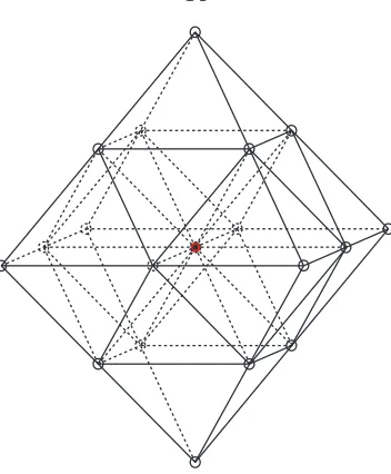
The 1-ring neighborhood domain of a regular vertex is shown in Fig. 2.4. As we will see in Chapter 4,

this 1-ring neighborhood is the support of a smooth subdivision scheme. For simplicity, we call this

neighborhoodME.

As shown in Fig. 2.5, the regular octet mesh has the face-centered cubic (FCC)structure which is the crystal structure of many chemical elements such as calcium and gold. The point group for the

FCC lattice isOh, which has 48 key symmetry operations:E, 8C3, 6C2, 6C4/3C2, i, 6S4, 8S6, 2σh

(25)

Figure 2.5: The topological configuration of the 1-ring domain around a regular vertex. This con-figuration has the well-known face-centered cubic structure.

when we write down the 1- and 2-form subdivision matrices later.

(1) 6C3 operations (2) 8C2 operations (3) 6C4 and 3C2

opera-tions

Figure 2.6: Some key symmetry operations for theOhpoint group

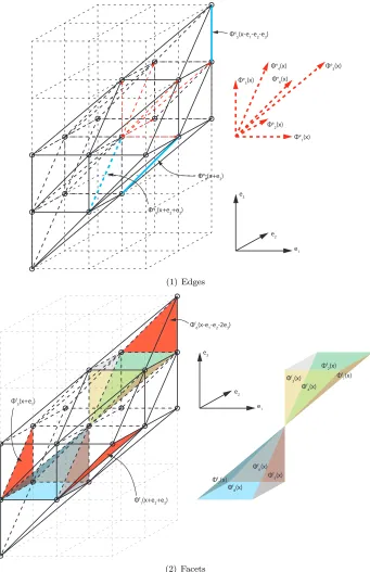
We can embed the regular mesh into a Z3-lattice as we did in Fig. 2.5. The drawback of this mapping is that the vertices here will not completely iterate all grid points in theZ3-lattice. However, as shown in Fig. 2.7, a one-to-one correspondence can be constructed between the vertices in the

regular octet mesh and theZ3-lattice. Furthermore, similar one-to-one mappings also exist for the edges, facets and cells of the regular mesh.

If we define a binary relation∼eon the edges of a regular octet meshMsuch that for∀e1, e2∈

Mr, e1∼ee2 if and only ife2 can be obtained by translatinge1 along theZ3-lattice, it is

straight-forward to show that∼eis an equivalence relation. Similarly, we can define ∼f,∼tand ∼o on the

facets, tetrahedra and octahedra ofM.

(26)

(1) Vertices (2) Edges (3) Facets

[image:26.612.111.536.119.535.2]

(4) Tetrahedra (5) Octahedra

(27)

Similarly, there are 8, 2 and 1 equivalence classes for facets, tetrahedra and octahedra, respectively.

Some examples of the translation transformation are shown in Fig. 2.8. Note that in the vertices,

edges and facets cases, if we remove one simplex, in order to reproduce all the simplices in the

corresponding equivalence class we need to translate using an offset that iterates whole Z3-lattice. However, in the tetrahedra and octahedra cases, the offset only needs to iterate 2×Z3, i.e., the translation always takes an even number of steps.

2.2 Subdividing the Octet Mesh

2.2.1 Linear 0-Form Subdivision

The linear subdivision proposed here is simply topological dyadic splitting without any geometric

smoothing. Specifically, the scheme is summarized in the stencil in Fig. 2.9.

We use two datasets as examples for the 0-form subdivision task. One isME, the 1-ring

neigh-borhood around a regular vertex (Fig. 2.10(1)). In order to test all the subdivision schemes on a

more exotic mesh, we also created a concave version ofME (denoted asMX, Fig. 2.10(2)).

Because the linear subdivision involves only splitting, the smoothness of the initial mesh does not

increase after subdivision. The volumetric domain associated with the mesh also does not change.

In other words, linear subdivision is a purely mesh generating process (Fig. 2.11).

2.2.2 Smooth 0-Form Subdivision

In order to derive the smooth subdivision stencil, we used techniques discussed in Section 3.3.2

and Section 3.4, where the theoretical framework of generating functions and the construction of

smoother subdivision schemes through convolution are introduced. Readers can skip the derivation

and return after reading these sections.

In the regular setting, subdivision schemes with higher regularity can be constructed from a given

subdivision scheme using convolution [44]. Specifically, based on the one-to-one mapping from the

regular mesh to theZ3-lattice (Fig. 2.7(1)), we can write down the generating function of the linear subdivision stencil:

c SL

v = 1 +

1 2

xyz+ 1

xyz +xz+

1

xz +x+

1

x+yz+

1

yz+y+

1

y +z+

1 z +1 6

xyz2+ 1

xyz2+xy+ y x+ x y + 1 xy . (2.10)

A smooth subdivision scheme can be obtained by convoluting the linear stencil with itself. In the

(28)

Φe 1(x)

Φe 2(x)

Φ₃(x) Φ₄(x)

Φe 5(x) Φ

e 6(x)

Φe 6(x+e2)

e₁ e₂ e₃

Φe 4(x+e2+e3)

(1) Edges

e₁ e₂ e₃

Φf 1(x)

Φf 2(x)

Φf 3(x)

Φf 4(x)

Φf 5(x)

Φf 6(x)

Φf 7(x)

Φf 8(x)

Φf 1(x+e2+e3)

Φf 6(x-e1-e2-2e3)

Φf 5(x+e1)

[image:28.612.153.494.62.589.2]

(2) Facets

(29)

1 1/2 1/2 1/6

1/6 1/6

1/6

Figure 2.9: 0-form linear subdivision stencil for three types of vertices: vertices in the coarse mesh, vertices introduced in the center of each edge and vertices introduced in the centroid of each octa-hedral cell

(1)ME dataset (2)MXdataset

Figure 2.10: Data files used in this chapter. Note that for theMX data, one side is concave.

Figure 2.11: 0-form linear subdivision results forME: initial mesh and meshes after 1∼4 times of

(30)

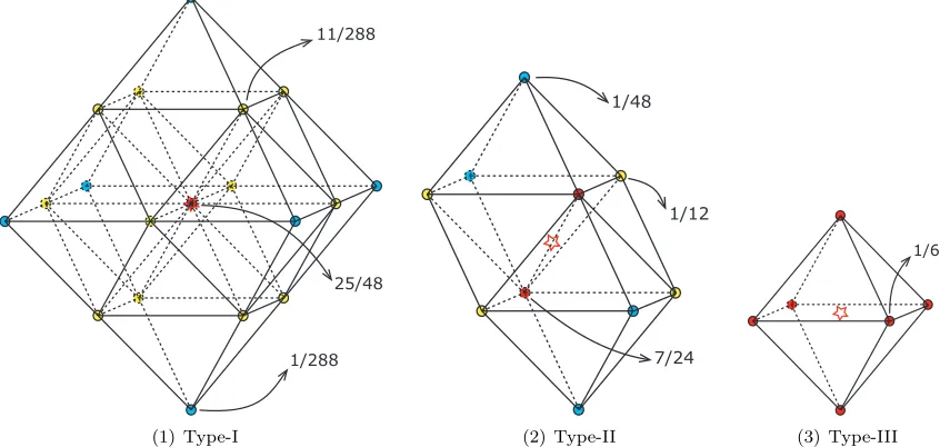
subdivision stencil is illustrated in Figure 2.12.

25/48 11/288

1/288

(1) Type-I

7/24 1/12 1/48

(2) Type-II

1/6

[image:30.612.111.534.153.354.2]

(3) Type-III

Figure 2.12: 0-form subdivision stencil in the regular setting. The star marks the position of the target vertex in the refined mesh. We use different colors to distinguish the vertices with different contributions in the coarse mesh.

The 0-form smooth subdivision scheme can be factorized into a simpler stencil defined on single

cells (Fig. 2.13). In practice, to find a vertex in the refined mesh, we must iterate over all the

adjacent cells (8 tetrahedra and 6 octahedra), calculate the new position of the vertex in each cell

and compute the arithmetic mean of these 14 positions.

Subdivision results for both datasets based on the smooth 0-form stencil just derived are shown

in Fig. 2.2.2. From the results we can clearly see that the smoothness of the mesh is improved every

time we subdivide the mesh. It can be proved that the smooth scheme generatesC2 _deformations

(31)

-1/16 _17/48

(1) Stencil in tetrahedron

3/8

1/12

7/24

[image:31.612.124.524.346.579.2]

(2) Stencil in octahedron

Figure 2.13: The 0-form linear subdivision after factorization

(1) Subdivision results ofME

(2) Subdivision results ofMX

Figure 2.14: 0-form smooth subdivision results for both data sets: initial mesh and meshes after 1

(32)

Discrete Differential Form

Subdivision over Volumetric

Domain

This chapter provides a thorough review of discrete differential geometry concepts related to the

3D volumetric domain 1- and 2-form subdivision problems. Section 3.1.1 reviews the definition and

properties of the simplicial complex; we extend the discussion to include the octahedral cells in

the octet mesh. Sections 3.1.2 and 3.1.3 discuss the discrete analogues of the integration operator,

differential forms and exterior derivatives. Section 3.2 introduces the definition of Whitney forms and

their realizations in tetrahedral and octahedral cells. Section 3.3 introduces the related theoretical

background behind the construction of the 1- and 2-form subdivision schemes for the volumetric

domain. Most of these theories are directly adapted from its analogues in the surface subdivision

theory. Section 3.4 briefly reviews on the commutative relations between subdivision operators that

is an analogue of Stokes’ rule in the continuous manifold. The theoretical background of constructing

smooth subdivision rule from linear subdivision scheme is also discussed here.

3.1 Basic Discrete Exterior Calculus

3.1.1 Simplicial Complexes and Boundary Operators

Simplices are the building blocks in the DDG framework. Anr-simplex σr is defined as the convex

hull ofr+ 1 geometrically independent points v0,· · · , vrand can be written as σr={x∈Rn| x=

Pr

i=0αivi whereαi ≥0 and Pri=0αi = 1}. σr can also be interpreted as a purely combinatorial

quantity represented by an (r+ 1)-tuple{v0,· · · , vr}. The elements in this (r+ 1)-tuple are called

vertices while the orderris called thedimension of the simplex.

Any subset of {v0,· · ·, vr} defines afacet of σr. Note that here “facet” generalizes the concept

(33)

of simplices that satisfies two additional conditions: (1) Every facet of a simplex in Kd is itself a

simplex; (2) The intersection of two simplices in Kd is either empty or an entire facet of each of

them. We define the dimension ofKd to be the highest of the dimensions of its contained simplices.

The collection of allr-simplices inKd is denoted asKrd.

A simplicial complex may be boundaryless; one example is a triangular tessellation of a sphere. If

a simplicial complex has a boundary, the boundary facets constitute a lower-dimensional simplicial

complex. Furthermore, for an interior vertex or point inside anr-dimensional simplicial complex, its

local neighborhood is homeomorphic to anr-sphere. In contrast, for the boundary vertex or point

inside any of the boundary simplices, its local neighborhood is homeomorphic to anr-semisphere.

In Chapter 2 we introduced the unstructured tetrahedral mesh (which, after one step of classical

subdivision, becomes an octet mesh). The tetrahedral mesh is an example of a 3D simplicial complex:

R, X1, X2 and X3 vertices are interior vertices while B1, B2 and B3 vertices are boundary vertices

(Section 2.1.1). One can convince oneself that the boundary of the whole mesh forms a 2D simplicial

complex without boundary. This is a consequence of Poincar´e’s lemma in the discrete domain.

The simplices in Kd are undirected. However, to simplify the discussions in this thesis and

facilitate the calculations of 1- and 2-form subdivisions, we extend the above definitions to the

oriented (or directed) context. If we introduce an equivalence relation among all the (r+ 1)-tuples

such that σr(1)∼σ(2)r if and only if one can be obtained by an even permutation of the other, then

all the r-simplices formed by verticesv0,· · ·, vr can be divided into two equivalence classes. Each

of these two classes is called an orientation. A simplex together with its orientation is called an

oriented simplex and is denoted as [v0,· · · , vr]. All the simplices mentioned below, if not mentioned

explicitly, are oriented. We use the same notationσrfor simplicity. While the orientation we assign

to a simplex is arbitrary and depends on the ordering of the vertices, the intrinsic orientations are

fixed and so are the associated geometric quantities. For example, suppose a simplex {vivj} is

immersed in a vector field, if the contour integral of the field along [vivj] yields Ithen the contour

integral of the field along [vjvi] yields−I. In other words, the 1-form coefficient associated with the

edge is bundled with the assumed orientation.

The boundary operator∂ applied to anr-simplex yields a sum of oriented (r−1)-facets of the simplex. Formally, ∂([v0,· · ·, vr]) = Pri=0(−1)i[v0,· · · ,vbi,· · ·, vr] where vbi indicates that the ith

vertex is missing from the tuple. A single tetrahedral cell is a useful example here. As shown in

Fig. 3.1, we assign each simplex an index. While the orientations of 0- and 3-simplices are always

positive, the 1-simplices’ orientation are indicated by the arrow in Fig. 3.1(2). For simplicity, for

2-simplices, if not mentioned explicitly, the orientations are assumed to be towards the exterior of

the tetrahedron. We emphasize again that, while we define the indexing and orientation rules in a

specific way and the use of “exterior” here makes the orientation coordinate dependent, these rules

(34)

[2] [3]

(1) Vertices

[4]

(2) Edges (3) Facets

Figure 3.1: Indexing rule for the tetrahedral cell

By specifying the indexing and orientation rules we can write down the boundary operator∂ in

a matrix format: it encodes the incidence relations between allr-simplices and all (r−1)-simplices inKd. For the example above we have

∂v₌

  

−1−1−1 0 0 0

1 0 0 −1 0 1

0 1 0 1 −1 0

0 0 1 0 1 −1

  , ∂e₌

      

1 0 −1 0

−1 1 0 0 0 −1 1 0

1 0 0 −1

0 1 0 −1

0 0 1 −1

      

, ∂f ₌

   1 1 1 1    (3.1)

which are boundary operators on 3-, 2- and 1-form, respectively. For example, theith column of∂v

records two ends of the edge, while theith column of∂e_{records three surrounding edges.}

One can easily verify that ∂∂ = 0 for the above example. This identity can be extended to

general simplicial complexes because, when we apply two boundary operations on ak-simplex, the

resulting (k−2)-simplices are paired up with opposite signs. This identity can be interpreted as stating that “the boundary of a boundary is empty”.

The concept of a simplicial complex can be extended to general unstructured meshes by allowing

non-simplicial polyhedrons to exist in the discrete manifold. Unlike the simplicial complex case

where we only have to specify the highest-dimensional simplices (e.g., from the configuration of the

tetrahedron, we are able to identify all facets and corresponding incidence relations with tetrahedral

cells, and then identify all edges and vertices), for a general unstructured mesh, we need to specify

all surrounding discrete submanifolds. For example, in the 3D case, for a polyhedronP we need to

specify that it is surrounded byn1 triangles and n2 quadrangles, etc. and also specify the

vertex-sequence of each polyhedron. For general non-simplicial polyhedra, the concept of orientation is also

induced from the equivalence classes based on the even permutation equivalence relation.

The generalization of the boundary operator is also straight forward. For an r-dimensional

(35)

B(P), then the boundary operator can be defined as

∂([v0,· · ·, v|P|]) =

X

Pi={˜v0,···,˜v|Pi|}∈B(P)

(−1)π([˜v0,···,v˜|_Pi|])_[˜_v0,_{· · ·} _,_v|_˜

Pi|]. (3.2)

Here, for any boundary facetPi, the vertex sequence is a subset of the vertex sequence of the parent

cellP. Here, we follow the convention that the order of the vertex sequence in each (k−1)-facet to be the same as in the parent cell. The orientation of the boundary submanifold is specified by

π∈ {−1,1}, which can be arbitrarily defined. For example, we can follow the convention that all the facets are pointing towards the exterior of the polyhedron or that the edges surround the facet

in a clockwise manner.

[1]

[2] [5] [3] [4]

[6]

(1) 0-form stencil

[1] [2]

[3] [4]

[5]

[6] [8]

[7]

[9] [10] [11]

[12]

(2) 1-form stencil

[1]

[2] [3] [4]

[5]

[6] [7] [8]

(3) 2-form stencil

Figure 3.2: Indexing rule for the octahedral cell

We want to write down the boundary operator for the octahedral cell. As shown in Fig. 3.2, the

0-, 1- and 3-simplices’ orientations follow the same conventions as in the tetrahedral case. Because

the octahedral cell is always adjacent to a tetrahedral case in the regular octet mesh, we define the

positive orientation of 2-simplices as the direction towards the interior of the octahedron. Unlike

the tetrahedral case, it is trickier to determine“interior” because a nondegenerate octahedron may

not be convex. As shown in Fig. 3.3, the interior of octahedron on the left side is well-defined. For

the other two octahedra, we need to pay more attention to detect the interior in practice.

If an octahedron is adjacent to a tetrahedron, because the orientation of the interface facet is

defined from the tetrahedron side, the interior of the octahedron can be easily identified. When the

octahedron is isolated or adjacent only to other octahedra, we use the following method to identify

the interior. Again, while this two-step algorithm is coordinate dependent, the intrinsic orientation

of the octahedron is fixed.

(36)

(1) Convex octahedron (2) Nonconvex octahedron (3) Another nonconvex octa-hedron

Figure 3.3: In a convex octahedral cell, for each facet, it is easy to tell which side is interior. However, we need a more complicated criterion to make such a judgement in the nonconvex octahedral cell.

count the number of intersections this half-line makes with all facets. If there is an even number of

intersections, this point is in the exterior of the cell, otherwise it is in the interior.

Step 2: Create a half-line li from p such that li intersects with facet fi at pi. li may have

intersections with other facets before pi. Assume pi is the ni-th intersection then we identify the

direction from whichli passes throughfi from the following decision matrix. The interior of the cell

and the induced orientation of the facet are then determined.

pis an interior point pis an exterior point

niis odd interior → exterior exterior → interior

niis even exterior → interior interior → exterior

(3.3)

Under this convention, the boundary operators for the octahedral cell can be written as

∂v₌

      

−1−1−1−1 0 0 0 0 0 0 0 0

1 0 0 0 −1 0 0 1 −1 0 0 0

0 1 0 0 1 −1 0 0 0 −1 0 0

0 0 1 0 0 1 −1 0 0 0 −1 0

0 0 0 1 0 0 1 −1 0 0 0 −1

0 0 0 0 0 0 0 0 1 1 1 1

       ,

∂e=

                

1 0 0 −1 0 0 0 0

−1 1 0 0 0 0 0 0

0 −1 1 0 0 0 0 0

0 0 −1 1 0 0 0 0

1 0 0 0 −1 0 0 0

0 1 0 0 0 −1 0 0

0 0 1 0 0 0 −1 0

0 0 0 1 0 0 0 −1

0 0 0 0 1 0 0 −1

0 0 0 0 −1 1 0 0

0 0 0 0 0 −1 1 0

0 0 0 0 0 0 −1 1

                

, ∂f =

(37)

3.1.2 Chains and Cochains

Given an oriented simplicial complex Kd, an r-chain is a linear combination of all r-simplices in

Kd (i.e., Pσ∈Kr

dc(σ)·σ where c(σ) ∈ R) and may be represented by a |K

r

d|-vector in which each

component corresponds to oner-simplex inKdaccording to some indexing rule. The collection of all

r-chains is denoted byCr(Kd). An important property of chains is that the boundary of anr-chain

is an (r−1)-chain. This is because boundary of an r-simplex is a linear combination of several (r−1)-simplices (with coefficients±1).

Recall that r-forms are linear mappings from an r-dimensional submanifold of a continuous

manifold to R. The collection of all the r-forms, Ωr₍_K

d), is a linear space. The discrete analogue

of an r-form is acochain which is defined as the dual of a chain. Specifically, we associate eachr -simplex with a real value. The set of these real values forms a|Kr

d|-vector that is called anr-cochain.

The collection of allr-cochains is a linear space and is denoted by Ωr

d(Kd). An “integral” is simply

the inner product of a chain and a cochain.

One can discretize an r-form on a continuous manifold by integrating it over each r-simplex

and associating the result (a scalar) with the simplex to form a cochain. Under this discretization

process, evaluating the inner products is consistent with classical integration, i.e.,

Z

¯

σr

ωr₌_h_ωr

d, σri (3.5)

whereωr

d∈Ωrd(Kd),ωdr∈Ωr(K),σr∈ Cr(Kd) and ¯σris exactly the same domain but interpreted as

a continuous submanifold immersed in the continuous domain.

It is clear that the above definition can be extended to the general unstructured polyhedron mesh.

Again we emphasize that, although we show how to discretize continuous forms through integration

over a submanifold, an underlying continuous manifold or differential form is not necessary: we

can assign arbitrary real values to each of the simplices. Indeed, we can also reverse the process.

As we can see in Section 3.2, given a cochain, a compatible continuous differential form can be

reconstructed through Whitney forms.

3.1.3 Exterior Derivatives and Coboundary Operators

The coboundary operator d is defined as the adjoint of the boundary operator ∂. Because the boundary of a chain cis also a chain, given a discrete form ωd the discrete integralhωd, ∂ciis well

defined andhdωd, ci=hωd, ∂ci. This is essentially the discrete analogue of Stokes’ theorem:

Z

P

ici∂σi

ω=hω, ∂(X

i

ciσi)i=hdω,

X

i

ciσii=

Z

P

iciσi

dω. (3.6)

(38)

0→Ω0

d(Kd)

d −→Ω1

d(Kd)

d

−→ · · ·−→d Ωn

d(Kd)→0. (3.7)

3.2 Whitney Forms over 3D Meshes

3.2.1 Whitney Forms

Whitney forms map from cochains to forms. Consider a simplicial complex Kd and the space of

r-forms Ωr₍_K

d). For any ω ∈ Ωr(Kd) and any r-chain c ∈ Cr(Kd), the integration R_cω can be

defined and is a linear function on chains. We denote this integration byR(ω)·c and name it the

de Rham map R: Ωr₍_K

d)→Ωrd(Kd).

Consider the inverse problem for 0-forms. The linear interpolation of discrete 0-forms to the

continuous domain is straightforward. We introduce the vertex-based interpolation basis (i.e., the

hat function): the basis functionφiassociated with vertexvi is a piecewise-linear function such that

φi= 1 atvi andφi= 0 at the rest of the vertices. Note thatPiφi = 1 andPidφi = 0.

Formally, the Whitney map is a linear map W : Ωr

d(Kd)→Ωr(Kd) such that for anyr-simplex

σr= [vi1· · ·vir]∈ Kd,

W σr=r! r

X

j=0

(−1)j−1_φ

ijdφi1∧ · · · ∧ddφij ∧ · · · ∧dφir. (3.8)

W σris called theWhitney form ofσr. LetWr(Kd) denote the space of the Whitneyr-forms onKd.

For anyr-simplex inKd the integration of the corresponding Whitney form is well-defined.

Consider Whitney forms on a 3-dimensional simplicial complex Kd. Assumeφi is the Whitney

0-form associated with the vertex [vi] in Kd, φij is the Whitney 1-form associated with the edge

eij = [vivj] in Kd, φijk is the Whitney 2-form associated with the facet fijk = [vivjvk] in Kd and

φijkl is the Whitney 3-form associated with the tetrahedrontijkl = [vivjvkvl] in Kd. Based on the

above definition of Whitney forms, we have

φij=φidφj−φjdφi (3.9)

φijk= 2(φidφj∧dφk+φjdφk∧dφi+φkdφi∧dφj) (3.10)

(39)

Using the fact thatφi+φj+φk+φl= 1 and dφi+ dφj+ dφk+ dφl= 0, the expression of the

Whitney 3-form can be simplified to:

φijkl= 6(φidφj∧dφkdφl−φjdφi∧dφkdφl+φkdφi∧dφjdφl−φldφi∧dφjdφk)

= 6[dφj∧dφk∧dφl−φj(dφi+ dφj)∧dφk∧dφl

−φk(dφi+ dφk)∧dφl∧dφj−φl(dφi+ dφl)∧dφj∧dφk]

= 6[dφj∧dφk∧dφl+φj(dφk+ dφl)∧dφk∧dφk

+φk(dφj+ dφl)∧dφl∧dφj+φl(dφj+ dφk)∧dφj∧dφk]

= 6dφj∧dφk∧dφl= 6dφk∧dφl∧dφi= 6dφl∧dφi∧dφj= 6dφi∧dφj∧dφk (3.12)

If we embed the simplicial complex into a metric space (here we useR3), we can visualize the Whitney 0-, 1-, 2- and 3-forms. Under the Euclidean metric, inside the tetrahedron, the Whitney

0-forms are piecewise-linear hat functions. More specifically, only the corresponding vertex has value

1 while other vertices are zero. Values inside the cell are linearly interpolated. Further, the 3-forms

are constant functions over the tetrahedron (proportional to the reciprocal of the volume). The

1-and 2-forms cases, together with the forms inside the octahedron, are not so straightforward. The

following sections addresses these difficulties.

3.2.2 Whitney Forms in the Tetrahedron

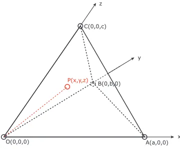
Now we start to calculate Whitney 1- and 2-form inside a 3-simplex T. We embed T into a

3-dimensional affine coordinate system shown in Fig. 3.4.

A(a,0,0) B(0,b,0)

C(0,0,c)

P(x,y,z)

O(0,0,0) x

[image:39.612.233.413.420.569.2]

y z

Figure 3.4: Mathematical setting for calculating Whitney forms in a 3-simplex

In this setting we have

φA=

x a, φB =

y

b, φC= z

c ⇒ dφA=

1

a(1,0,0), φB=

1

b(0,1,0), φC=

1

(40)

Furthermore, the Whitney 2-form vector with respect to the facet ∆ABC is

φABC = 2φAdφB∧dφC+ 2φBdφC∧dφA+ 2φCdφA∧dφB =

2

abc(x, y, z). (3.15)

The vector field associated with this result is shown in Fig. 3.5(2). For each vector,φABC is parallel

to OP. Similar to the 1-form case, the integral of the vector field on all facets only yields nonzero

value on ∆ABC.

A

B

(1) 1-form

B A

C

(2) 2-form

Figure 3.5: Whitney forms in the tetrahedral cell

3.2.3 Whitney Form in the Octahedron

Unfortunately, Whitney forms were originally only defined on simplices and there is no closed-form

formula for the Whitney forms inside the octahedron. However, we can use linear 1- and 2-form

subdivision (Section 4.1) to approximately model the Whitney forms in the octahedron. We only

present the results here. Details of this method are discussed in Appendix A.3.2. As one can see

from Fig. 3.6, integrating the vector field on all edges or facets yields nonzero value only on the edge

(41)

B A

(1) 1-form

B

A C

(2) 2-form

Figure 3.6: Whitney forms in the octahedral cell

3.3 Cochain Subdivision

3.3.1 Subdividing the Vector Field

Refinable functions play a vital role as reconstruction bases in subdivision theory and scaling

func-tions in wavelet theory. These funcfunc-tions have a certain level of self-similarity properties. For example,

a single-variable functionf is said to be refinable with respect to the maskh if it satisfies the

re-finement equation (also known as the dilation equation)f(x) =P_k_∈_Zhkf(2x−k). The refinement

equation can be interpreted as the discrete convolution with the discrete mask h followed by a

dilation operation.

Take Whitney 0-forms as an example. In one dimension, these are just piecewise-linear hat

functions (Fig. 3.7(1)) which satisfy a simple two-scale dilation relation (f(x) = 1

2f(2x−1) + f(2x)+1

2f(2x+1), Fig. 3.7(2)) that yields piecewise-linear interpolation if we subdivide the function

infinitely often.

(1) Coarse level, 1D (2) Refined level, 1D (3) Coarse level, 2D (4) Refined level, 2D

(42)

are induced by piecewise-linear functions, the refinement equation for Whitney 1-forms result in a

piecewise-linear interpolation of vectors valued at vertices.

Forf(x_{) on}_R3_{, the refinement equation can be similarly defined as}

f(x) = X k∈Z3

hkf(2x−k). (3.16)

Although the piecewise-linear hat function in 3D domain can no longer be visualized, the concept

is identical. Similarly, the refinement equations for 1- and 2-forms lead to a piecewise-linear

inter-polation of vectors valued at vertices. One can observe these facts by inspecting results in Fig. 3.5.

However, such subdivision rules for vector fields have at least two drawbacks. First, for the

octahedral cell, the refinement relation is not obvious: we can no longer utilize a piecewise-linear

interpolation of vectors valued at vertices. Second, vector fields rely not only on the topological

structure of the mesh, but also on the metric space the mesh embedded in. What we really want is the

refinement rule of ther-form coefficients which lie onr-simplices and is based only on the topological

structure. Next, based on the refinement relation for vector fields (i.e., linear interpolation), we

introduce the concept and notation of the refinement rules of the form coefficients.

1/2

1/2 1/2

-1/2

(1) Whitney subdivision stencil for 1-forms in the tetrahedral cell

1/4

1/8

1/8 1/8

(2) Whitney subdivision stencil for 2-forms in the tetrahedral cell

Figure 3.8: Linear subdivision schemes for vector fields associated with Whitney 1- and 2-forms in the tetrahedral cell

The 1- and 2-form subdivision rules calculated from the linearly interpolated vector field are

illustrated in Fig. 3.8. The stencil is calculated by integrating the vector field along the simplices in

the refined mesh and is called the Whitney subdivision scheme or linear subdivision scheme. This will serve as the basis of a smoother subdivision scheme which we construct later. The subdivision

rule for octahedral cells is still missing here. Assume the octahedral cells also have a refinement

Discrete Differential Form Subdivision and Vector Field Generation over Volumetric Domain

Generation over Volumetric Domain

Jinghao Huang

Acknowledgements

Contents

List of Figures

Chapter 1

Introduction

1.1

Classical Vertex-Based Subdivision on Surfaces

1.2

Discrete Differential Geometry

1.3

Edge-Based Subdivision on Surface

1.4

Subdivision in the Volumetric Domain

1.5

Overview and Contribution

Classical 0-Form Subdivision in the

Volumetric Domain

2.1

Geometric and Topological Properties of the Octet Mesh

2.1.1

Types of Vertices in the Octet Mesh

2.1.2

Properties of the Regular Mesh

2.2

Subdividing the Octet Mesh

2.2.1

Linear 0-Form Subdivision

2.2.2

Smooth 0-Form Subdivision

Discrete Differential Form

Subdivision over Volumetric

Domain

3.1

Basic Discrete Exterior Calculus

3.1.1

Simplicial Complexes and Boundary Operators

3.1.2

Chains and Cochains

3.1.3

Exterior Derivatives and Coboundary Operators

3.2

Whitney Forms over 3D Meshes

3.2.1

Whitney Forms

3.2.2

Whitney Forms in the Tetrahedron

3.2.3

Whitney Form in the Octahedron

3.3

Cochain Subdivision

3.3.1

Subdividing the Vector Field