https://doi.org/10.5194/hess-22-4725-2018 © Author(s) 2018. This work is distributed under the Creative Commons Attribution 4.0 License.
Including effects of watershed heterogeneity in the curve
number method using variable initial abstraction
Vijay P. Santikari and Lawrence C. Murdoch
Department of Environmental Engineering and Earth Sciences, Clemson University, Clemson, SC 29634, USA Correspondence:Vijay P. Santikari ([email protected])
Received: 15 October 2017 – Discussion started: 8 November 2017
Revised: 21 May 2018 – Accepted: 25 June 2018 – Published: 10 September 2018
Abstract. The curve number (CN) method was developed more than half a century ago and is still used in many water-shed and water-quality models to estimate direct runoff from a rainfall event. Despite its popularity, the method is plagued by a conceptual problem where CN is assumed to be constant for a given set of watershed conditions, but many field obser-vations show that CN decreases with event rainfall (P). Re-cent studies indicate that heterogeneity within the watershed is the cause of this behavior, but the governing mechanism re-mains poorly understood. This study shows that heterogene-ity in initial abstraction,Ia, can be used to explain how CN
varies withP. By conventional definition,Iais equal to the
cumulative rainfall before the onset of runoff and is assumed to be constant for a given set of watershed conditions. Our analysis shows that the total storage in Ia (IaT) is constant,
but the effective Ia varies withP, and is equal to the filled
portion ofIaT, which we call IaF. CN calculated using IaF
varies with P similar to published field observations. This motivated modifications to the CN method, called variableIa
models (VIMs), which replaceIawithIaF. VIMs were
evalu-ated against conventional models CM0.2 (λ=0.2) and CMλ (calibratedλ) in their ability to predict runoff data generated using a distributed parameter CN model. The performance of CM0.2 was the poorest, whereas those of the VIMs were the best in predicting overall runoff and watershed heterogene-ity. VIMs also predicted the runoff from smaller events bet-ter than the CMs and eliminated the false prediction of zero-runoffs, which is a common shortcoming of the CMs. We conclude that including variableIaaccounts for
heterogene-ity and improves the performance of the CN method while retaining its simplicity.
1 Introduction
The estimation of runoff from a rainfall event is of primary importance in applied hydrology. It is necessary in the engi-neering design of small structures, post-event appraisals, en-vironmental impact work, and other applications (Hawkins, 1993). One of the most popular techniques used for this pur-pose is the curve number (CN) method, which has been in use for more than half a century (D’Asaro and Grillone, 2012; Hawkins et al., 2008; Kent, 1968; Ponce and Hawkins, 1996; Rallison and Miller, 1982; Soil Conservation Service, 1956, 1972). The method uses a parameter called curve number, which is assumed to depend mainly on land cover, soil types, and antecedent conditions within a watershed.
This diminishes the accuracy of its runoff predictions (e.g., Soulis and Valianzas, 2012).
The objective of this work is to improve the event-scale lumped-parameter application of the CN method by describ-ing an approach for incorporatdescrib-ing the spatiotemporal varia-tions of CN. The investigation is described in two papers, which build on Santikari (2017). In this paper, effects of spa-tial variation of CN (heterogeneity) at the watershed scale are analyzed. Insights gained from this analysis are used to create modified models that account for heterogeneity. The modified models are evaluated using the runoff generated by a distributed parameter model applied to a hypothetical het-erogeneous watershed. In a companion paper (Santikari and Murdoch, 2018) and in Santikari (2017), the modified mod-els are refined by including an approach that accounts for the temporal variation of CN using antecedent moisture. The refined models, which account for spatial and temporal vari-ability, are then evaluated using data from real watersheds. 1.1 Background
The CN method assumes that a rainfall event produces runoff (Q) when the event rainfall (P) exceeds the initial abstraction (Ia). Ia includes interception storage (by tree
canopy, roof tops, and such), early infiltration, and surface depression storage. The effective rainfall, P−Ia, is
parti-tioned betweenQand further infiltration (F). This is given by mass balance as
P −Ia=F+Q∀P ≥Ia. (1)
BothF andQare zero whenP≤Ia, and both increase with
P when P > Ia. It is assumed that F has an upper limit,
which is referred to as the potential maximum retention (S). In other words,Sis the total storage available for infiltration after the runoff begins.
The conceptual basis that defines the curve number method comes from the following assumption (Hawkins et al., 2008; NRCS, 2003; Ponce and Hawkins, 1996; Rallison and Miller, 1982; Woodward et al., 2002):
Q P−Ia
=F
S, (2)
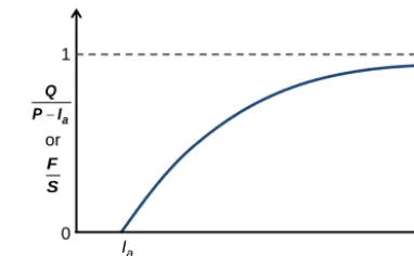
i.e., the runoff coefficient (left-hand side) is equal to the frac-tion of storage filled in S (right-hand side). Equation (2) is developed using the reasoning that the equality holds at the end points (P≤IaandP → ∞) (Hawkins et al., 2008;
Ral-lison and Miller, 1982; Woodward et al., 2002) and that the behavior of both ratios in the intermediate range is essen-tially the same (Fig. 1). WhenP≤Ia, bothQandF are zero
and therefore the ratios on either side of Eq. (2) are zero. WhenP > Ia, both ratios increase withP, whereas their rate
of increase diminishes. At the limit of P→ ∞, both ratios approach unity.
P 1
Ia 0
a Q P I
F S
[image:2.612.330.521.68.186.2]or
Figure 1.Presumed variation of the ratios in Eq. (2) with event rain-fall (P).Qis event runoff,Iais initial abstraction,Fis cumulative infiltration after runoff begins, andSis potential maximum reten-tion (modified from Rallison and Miller, 1982, Fig. 2).
To eliminate the need for an independent estimation ofIa
(Ponce and Hawkins, 1996; Rallison and Miller, 1982), it is assumed that
Ia=λS, (3)
whereλ is a dimensionless parameter called the initial ab-straction ratio. Early field data suggested an optimum value ofλ=0.2 (Soil Conservation Service, 1956). However, more recent studies (Hawkins et al., 2008; Woodward et al., 2003) suggest thatλ=0.05 is more appropriate. Using Eqs. (1)– (3),IaandF can be eliminated to give
Q=0∀P ≤λS, Q= [P−λS]
2
P +(1−λ)S ∀P > λS. (4)
Since the value ofλis usually fixed (at 0.2 or 0.05), Eq. (4) requires only one parameter,S, which varies within the range 0≤S≤ ∞.
For convenience (Hawkins et al., 2008; Ponce and Hawkins, 1996),S (units in mm) is mapped onto a dimen-sionless parameter called the curve number as
CN= 25 400
254+S (5)
so that CN is 100 when S is zero, but approaches zero as Sapproaches infinity. In practice, whenλ=0.2, CN ranges from around 30 (for vegetated surfaces with highly perme-able soils) to close to 100 (for impermeperme-able surfaces or soils) (USDA, 1986). Tabulated CN values for various land uses, soil types, and management scenarios are available in hand-books and manuals (NRCS, 2003; USDA, 1986). CN can also be determined from field data by solving Eq. (4) forSas S= 1
2λ2 h
2λP+(1−λ)Q−p(1−λ)2Q2+4λP Qi (6)
BC5
P (mm)
0 30 60 90 120 150
CN
40 60 80 100
BC1
P (mm)
0 30 60 90 120 150
CN
40 60 80 100
BC5
P (mm)
0 30 60 90 120 150
I a (mm)
0 25 50 75
BC1
P (mm)
0 30 60 90 120 150
I a
(mm)
0 25 50 75 (a)
(c)
(b)
(d)
R2 = 0.89 R2 = 0.93
[image:3.612.99.489.78.351.2]0.64 P - 0.002 P2 0.67 P - 0.002 P2
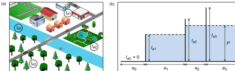
Figure 2.Variation of CN (λ=0.2) withP in watersheds(a)BC5 and(b)BC1, near Greenville, SC. Variation ofIawithP in(c)BC5 and (d)BC1 (see Santikari, 2017, or Santikari and Murdoch, 2018, for study area description). Best-fit curves forIaare quadratic functions ofP with zero intercept. Corresponding best-fit curves for CN were derived from those ofIausing Eqs. (3) and (5).
The curve number method is appealing because it is based on an intuitive concept (Eq. 2), relies on only one parame-ter, has a large body of literature (Hawkins et al., 2008), and has a comprehensive database (NRCS, 2003; USDA, 1986). It has been included in many watershed and water-quality models such as SWAT (Soil and Water Assessment Tool) (Neitsch et al., 2005), CREAMS (Chemicals, Runoff and Erosion from Agricultural Management Systems), GLEAMS (Groundwater Loading Effects of Agricultural Manage-ment Systems) (Knisel and Douglas-Mankin, 2012), An-nAGNPS (Annualized Agricultural Non-point Source Pol-lution Model) (Bingner et al., 2011), EPIC (Environmen-tal Policy Integrated Climate), APEX (Agricultural Pol-icy/Environmental Extender) (Wang et al., 2012), and Hy-droCAD (HyHy-droCAD, 2015). A physically based modeling framework, such as the diffusive-wave approximation for overland flow coupled with the Richard’s equation for unsat-urated subsurface flow, e.g., Panday and Huyakorn (2004), may improve accuracy and resolution of model predictions compared to the CN method, when the necessary input data, expertise, and computing resources are available. However, the CN method will likely remain popular for many ap-plications in runoff modeling because of its ease of use, wide knowledge base, and less demand on computational re-sources than many physically based models.
1.2 CN variation withP
In watersheds showing a standard behavior, CN was treated as an asymptotic function ofP as
CN=CN∞+(100−CN∞) e−kP, (7)
where CN=CN∞is the asymptote andkis a calibration
pa-rameter (Hawkins, 1993). CN∞is the smallest possible value
of CN for a watershed and is approached only at large val-ues of P. To develop Eq. (7), measured values of Q, ide-ally for a large range of values ofP, are needed. The usual procedure involves “frequency matching” the data (Hawkins, 1993), i.e., sorting the values ofPandQseparately, and pair-ing them accordpair-ing to their rank. CN for each pair is then cal-culated using Eqs. (5) and (6). Frequency matching reduces the scatter of data points around the best-fit curve in a CN vs.P plot.
A standard behavior of CN was also observed in two wa-tersheds (BC5 and BC1) near Greenville, South Carolina, USA (Fig. 2a and b). In these watersheds, CN (calculated usingλ=0.2) decreased from 97 to 50 asP increased from 2 to 128 mm. The data were characterized by a modest scat-ter (R2=0.9) about the best-fit curve based on a quadratic function of P. Description of these watersheds is given by Santikari (2017) and Santikari and Murdoch (2018). The jus-tification for using quadratic functions follows from the anal-ysis of heterogeneity presented in Sect. 2.
The approach used in Fig. 2a and b avoids the commonly used frequency matching (e.g., Hawkins, 1993). Each CN value in the plot was calculated using theP−Qpair from the same storm event. Frequency matching would signifi-cantly reduce the scatter in the plot, but it would also down-play the importance of CN variation due to antecedent condi-tions. Reducing the scatter by accounting for antecedent con-ditions, e.g., using antecedent moisture (Mishra et al., 2006), is a better approach.
The hypotheses given by Hawkins (1993) are valid, but in-sufficient to explain the standard and complacent behaviors. It may be true that small rainfalls produce runoff only un-der wet (large CN) conditions and therefore only the large CN values are recorded. However, if one has a large enough sample of storms, some of the larger storms also must have occurred during wet conditions. For the larger storms, there-fore, one would expect to see the whole spectrum of CN val-ues ranging from the largest to the smallest. However, this is not the case. As P increases, the values of CN decrease consistently (Fig. 2a and b).
1.3 Heterogeneity as a cause of CN variation withP
Soulis and Valiantzas (2012) hypothesized that the observed variation of CN withP in the standard and complacent cases is a consequence of watershed heterogeneity. They assumed a hypothetical heterogeneous watershed with two subareas characterized by different CNs. They then calculated the watershed runoff, for a range of values of P, as the area-weighted average of the runoffs from the subareas.
Water-shed CN calculated using this runoff varied withP akin to the standard behavior. The shape of the synthetically gener-ated CN vs.P curve could be matched with the observations by adjusting the areas of the subareas and their respective CNs. This idea can also be extended to multiple subareas so that the heterogeneity within a watershed can be repre-sented more accurately. However, this could lead to prob-lems of over-parameterization, uniqueness, and non-convergence as pointed out by Soulis and Valiantzas (2012). In a later paper, Soulis and Valiantzas (2013) suggested using spatial information on land cover and soils to delin-eate the areal extent of subareas and constrain their respective CNs. This approach would reduce the number of calibrated parameters by half because it only requires the calibration of the CNs for the subareas. In essence, the multiple-subarea approach is similar to a distributed modeling approach that calculates the watershed runoff as the area-weighted average of the runoffs from the subareas, e.g., SWAT (Gassman et al., 2007). The approach used by Soulis and Valiantzas (2013) attempts to match the observed and simulated values of CN, whereas that used by SWAT attempts to match the observed and simulated values ofQ. Since CN and Qare uniquely related for given values ofP andλ, these approaches are equivalent. A major implication of the work of Soulis and Valiantzas (2013) is that a distributed modeling approach can account for the standard and complacent behaviors of CN.
Using a single value of CN independent ofP in a hetero-geneous watershed can cause a systematic error inQand lead to poor predictive ability of the method. This is because when CN is constantQmay be underestimated for smallP and overestimated for largeP (e.g., Soulis and Valianzas, 2012, 2013). This problem can be addressed either by treating CN as a function ofP, e.g., asymptotic fitting (Hawkins, 1993), or by using a distributed modeling approach that accounts for heterogeneity in sufficient detail, e.g., SWAT (Gassman et al., 2007) or Soulis and Valianzas (2013). An understand-ing of the mechanism of how watershed heterogeneity leads to the variation of CN withP is also important. It could help in accounting for this variation without resorting to fine dis-cretization or over-parameterization of the CN method. To accomplish this, an analysis of the effect of heterogeneity on IaandSis performed, which can then be used to understand
the effect on CN.
2 Reevaluation of initial abstraction
The quantities CN,Ia, andSare considered to be the
can expect that they too vary withP but inversely to that of CN. The calculated values ofIa(using Eqs. 3, 6, andλ=0.2)
for watersheds BC5 and BC1 near Greenville, SC, increase withP and appear to approach a constant at large values ofP (Fig. 2c and d). A plot ofS vs.P would be similar to theIa
vs.P plot, with theycoordinate scaled by 1/λ.
To evaluate the link between heterogeneity in Ia and its
variation with P, we looked at how the effective Ia of a
heterogeneous watershed is determined and whether it is af-fected by the magnitude ofP. Our analysis shows that there is an inconsistency between the theoretical definition of Ia
and its calculated value at the watershed scale. It also shows how heterogeneity can causeIato vary withP and how this
relates to variations ofSand CN withP. 2.1 Problems with the current usage ofIa
By the theoretical definition ofIa, if runoff is detected in the
hydrograph, it is assumed thatIahas been met for the
water-shed. Watersheds are heterogeneous combinations of various land-use–soil–slope complexes. These are referred to as hy-drologic response units (HRUs) in SWAT (Gassman et al., 2007), and the same term is also used here. Each HRU is assumed to be homogeneous and is characterized by repre-sentative values of CN (CNi) andIa (Iai). During a rainfall event, the HRU with the smallest of the Iai values will be the first to generate runoff. Assuming that this runoff reaches the watershed outlet, by definition, the Ia of the watershed
should be equal to the smallest of theIai values. This could even be zero if the watershed has surfaces such as open water bodies that cannot abstract the rainfall.
However, it is difficult to detect the exact moment of gen-eration of runoff and determine the corresponding value of Ia, which is equal to the cumulative precipitation at that
mo-ment. There have been studies (Shi et al., 2009; Woodward et al., 2003) that tried to determineIafrom hydrographs. A
problem with this approach is that there can be a time lag between runoff generation in headwaters and its detection at gauging station. Rainfall that occurs during this time lag is also included in Ia, leading to its overestimation. Another
possible approach would be to collect observations from a large number of rainfall events and take Ia to be equal to
the smallest P that produced runoff. This would eliminate the problem with the lag time, but Qneeds to be insignifi-cant to reduce the error inIa. It should also be noted thatIa
determined this way is only representative of the antecedent conditions of the smallest event that produced runoff.
It may be difficult to measure Ia directly, but it can be
calculated for any event using Eqs. (6) and (3). However, in medium to large rainfall events, even the HRUs with larger values ofIai will contribute toQ. Therefore, the calculated value of Ia in these events will also be influenced by the
larger values of Iai. So, the calculatedIa tends to be greater
than the smallest of the Iai values. Moreover, it can be ex-pected to increase withP as increasingly larger rainfalls
gen-erate runoff from HRUs with increasingly larger values of Iai. Thus, there is an inconsistency between the definition of Iaand its calculated value at the watershed scale.
Spatial-scale effect onλ
Strictly adhering to the definition ofIaat the watershed scale
may also cause a spatial-scale effect on λ. Let us refer to the CN of the watershed as CNW and toIa asIaW. One of
the common ways to determine CNWis to calculate it as the
area-weighted average of the CNivalues (NRCS, 2003) as
CNW=
n X
i=1
aiCNi, (8)
whereai is the fractional area of the ith HRU. Note that the fractional areas must add up to unity. By definition, IaW is equal to the smallest of theIai values. Therefore, if Ia1< Ia2<. . .< Ian, then
IaW=Ia1. (9)
From Eqs. (3) and (5) it can be shown that CN andIa are
related as CN= 25 400
254+Ia λ
. (10)
If all the HRUs are assumed to have the same λ=λi, Eqs. (8)–(10) lead to
CN1>CN2> . . . >CNn
CNW<CN1
IaW
λW
>Ia1 λi ,
λW< λi, (11)
whereλWis the effective initial abstraction ratio of the
wa-tershed. Therefore, ifλis assumed to be the same among the component HRUs, it will have a smaller value at the water-shed scale. This implies thatλdecreases with increasing spa-tial scale. Therefore, settingλconstant, equal to 0.2 or 0.05, for all the spatial scales contradicts the definition ofIa. In
any case, it is probably more accurate to calculate runoff at the HRU scale (Qi) and take the area-weighted average of Qi values, rather than take the area-weighted average of the CNi values and calculateQat the watershed scale. It is also more appropriate becauseQis runoff per unit area, whereas CN is a dimensionless index variable.
The inconsistencies in the usage ofIaare a direct result of
heterogeneity in a watershed. Moreover, heterogeneity also appears to be responsible for the variation of IaW withP
(Fig. 2c and d). To verify this, a relationship betweenIaW
(a) (b)
Ia0
Ia1
Ia2
Ia3
a1 a2
a0 a3
Ia1
Ia2 Ia3
Ia0= 0
[image:6.612.105.495.67.186.2]P
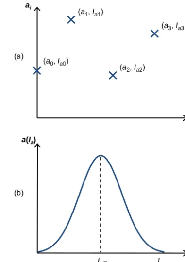
Figure 3.Spatial distribution ofIain a heterogeneous watershed.(a)Iai values of various HRUs mainly characterized by their land use types (Ia0=0< Ia1< Ia2< Ia3);(b)conceptual model in which each HRU is represented by a bin with height=Iai, width=ai, and unit thickness; shaded area indicates the filled portion during an event with rainfall=P.
2.2 Iain a heterogeneous watershed
Consider a watershed with four HRUs mainly character-ized by their land use types, viz. open waterbody (Ia0),
ur-ban area (Ia1), park (Ia2), and forest (Ia3) (Fig. 3a), such
that Ia0=0< Ia1< Ia2< Ia3. An open waterbody generates
runoff during every rainfall event. Other land use types gen-erate runoff depending on the magnitude of the rainfall, with land uses of largerIai values requiring larger magnitudes. If each land use type is assumed to be directly connected to the drainage network, the number of land use types contributing to the runoff, in other words the runoff contributing area, in-creases with rainfall. This process can be conceptualized by representing the storage distribution ofIaas a series of bins
where each bin corresponds to a HRU (Fig. 3b). The height and the width of a bin are given byIai andai, respectively, and all bins have unit thickness. In a rainfall event, only the bins with Iai≤P are fully filled and contribute to runoff, whereas the others are partially filled and do not contribute to runoff. The total amount of filled storage inIa(shaded area
in Fig. 3b) increases withP until it reaches a constant value when all the bins are fully filled and the whole watershed is contributing to the runoff.
Consider a general case of a heterogeneous watershed with n+1 HRUs such that
Ia0=0< Ia1< Ia2< . . . < Ian, (12)
where Ia0 represents open water bodies and other surfaces
that cannot abstract rainfall. The areal average of the total initial abstraction (IaT) is given by
IaT=
n X
i=0
aiIai. (13)
In a rainfall event, all the HRUs withIai≤P have their ini-tial abstractions completely filled while the others are par-tially filled. Just by analyzing the runoff for that event, it is impossible to quantify the magnitudes of Iai in HRUs that are partially filled. Because these HRUs have not contributed
to the runoff, all that can be said is that theirIai values are greater thanP, but their magnitudes remain unknown. How-ever, the information on the magnitudes ofIai in HRUs that are completely filled should be present in the runoff data. In other words, it takes larger rainfalls to fill larger values ofIai and gather information about their magnitude.
Then what is the effective initial abstraction of the water-shed for a given rainfall event? Consider an event where the rainfall falls within the range:Iam≤P < Ia(m+1). HRUs with Iai≤Iamhave their initial abstractions completely filled and produce runoff, whereas HRUs withIai≥Ia(m+1)have their initial abstractions partially filled up to the level ofP and do not produce runoff. The areal average of the filled portion (includes completely filled as well as partially filled HRUs) of the initial abstraction is given by
IaF=
m X
i=0
aiIai+ 1− m X
i=0
ai !
P . (14)
The first term on the right-hand side of Eq. (14) represents completely filled HRUs. The second term represents partially filled HRUs, all of which are filled to the level ofP. Note that IaTis the areal average of total initial abstraction, whereasIaF
is the areal average of the filled portion. Therefore, IaF< IaT∀P < Ian,
IaF=IaT∀P ≥Ian. (15)
The conceptual model presented in Fig. 3 as well as in Eqs. (14) and (15) is intuitively appealing and also hints at the possibility thatIaWmay be equal toIaF. This is because
IaFincreases withP and approaches a constant value (IaT),
similar to the observations in Fig. 2c and d. Equation (14) is also consistent with a distributed parameter model applica-tion of the CN method as described in Sect. 3.
2.3 Variation ofIaFwithP
To investigate the variation ofIaFwithP, Eqs. (14) and (15)
P P = Ia1
IaF
[image:7.612.70.260.71.187.2]P = Ia2 P = Ia3 IaT
Figure 4.Variation ofIaF(Eqs. 14 and 15) withP for the scenario presented in Fig. 3.
plot ofIaFvs.P (Fig. 4) shows thatIaFincreases withP and
becomes constant (IaF=IaT) at large values ofP (P≥Ia3).
The kink points joining the line segments occur when the initial abstraction of one of the HRUs becomes completely filled. At these points, P is equal to one of the Iai values. In between these points (Iam< P < Ia(m+1)), the relationship betweenIaFandP is linear with a slope of
1−
m P
i=0
ai
. The slope abruptly changes across the kink points. It decreases withmand becomes zero whenm=n. The maximum value the slope can take is unity. This occurs with the line seg-ment passing through the origin, when HRUs with zero ini-tial abstraction are absent (i.e., a0=0). When these HRUs
are present, however, the origin itself is a kink point where the slope abruptly jumps from unity to 1−a0.
The analysis presented so far represents a discrete case where each HRU is homogeneous and has a finite area. The values of Iai vary discontinuously across the HRUs. Their areal distribution can be represented by a plot of ai vs. Ia
(Fig. 5a). The smaller the area of HRUs, the more numer-ous they are and the more accurate the representation of the heterogeneity within the watershed is. The most ideal repre-sentation would occur when the HRUs shrink to points. Then the values ofIai within the watershed vary continuously and therefore can be represented by a probabilistic distribution of areal occurrence (Fig. 5b). It is impractical to characterize the watershed at such fine scale, but it is worth understanding the properties of the initial abstraction at the finest resolution first and then making assumptions or simplifications later to suit the practical needs.
For the case of a continuous distribution of Ia, Eq. (14)
takes the form
IaF=
P Z
0
Iaa (Ia)dIa+
1− P Z
0
a(Ia)dIa
P , (16) wherea(Ia)is the probability density function of areal
occur-rence ofIa. The fractional area with initial abstraction=Iais
given bya(Ia)dIa. The upper limit of the integrals is set toP
because the last initial abstraction to completely fill up would
Ia ai
(a0, Ia0)
(a)
(b)
Ia a(Ia)
IaT Ia,max
(a1, Ia1)
(a2, Ia2)
(a3, Ia3)
Figure 5.Representing areal distribution ofIawithin a watershed (a)discrete case and(b)continuous case.
be equal toP. The areal average of total initial abstraction, IaT, is given by
IaT=
Ia,max Z
0
Iaa (Ia)dIa, (17)
where Ia,max is the maximum value of Ia within the
wa-tershed. Thus, IaT is equal to the mean of the distribution
(Fig. 5b). Equation (15) then becomes IaF< IaT∀P < Ia,max,
IaF=IaT∀P ≥Ia,max. (18)
Unlike the discrete case, the slope of the IaF curve for
the continuous case decreases smoothly with increasingP (Fig. 6). This is because the line segments in the discrete case (Fig. 4) shrink to points in the continuous case. It follows from Eq. (16) that
dIaF
dP
P=0 =1, dIaF
dP
P≥Ia,max
=0. (19)
Thus, theIaF curve is bounded by a line of slope=1
[image:7.612.329.520.73.343.2]P IaF
Ia,max 0
IaT
[image:8.612.327.524.68.206.2]No-runoff line, slope = 1
Figure 6.Variation ofIaFwithP for a continuous distribution such as the one shown in Fig. 5b.
as the no-runoff line because along this lineIaF=P. When
the whole watershed is represented by a single HRU, the IaF curve coincides with the no-runoff line until IaF=IaT.
A comparison of Figs. 6 to 2c and d strengthens the case that IaWis equal toIaF.
2.4 Variation of CNWwithP
Let us hypothesize thatIaW=IaF; i.e., the effectiveIa of a
watershed is equal to the area-weighted average of the filled portion of the initial abstraction. Then, if Eq. (10) is written for CNW,Ia can be replaced by IaF. Substituting Eq. (16)
in Eq. (10) gives CNW as a function of P. When plotted
againstP, CNWstarts at 100 whenP =0 and then decreases
with increasingP (Fig. 7).
Differentiating Eq. (10) and using Eq. (19) gives d(CNW)
dP
P=0 = −10
λ, d(CNW)
dP
P≥Ia,max
=0, (20)
where the constant 10 has units of 1/in. Thus, the CNW
vs. P curve is at its steepest atP=0 and flattens with in-creasingP, and it becomes constant whenP≥Ia,max. This
constant, CNT, is the smallest value CNWcan take and
cor-responds to the caseIaF=IaT, when the initial abstractions
of all the HRUs are fully filled. CNW as a function ofP is
bounded by a curve corresponding to the conditionP=IaF,
the no-runoff line, and a line of slope=0 with the intercept equal to CNT(Fig. 7).
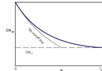
The shape of the CNWvs.P curve (Fig. 7) generated
us-ing Eqs. (10) and (16) is quite similar to the best-fit curves from field observations (Fig. 2a and b). Nearly 95 % of the watersheds evaluated in the previous studies (D’Asaro and Grillone, 2012; Hawkins, 1993) also had responses identi-cal to Fig. 7, supporting the hypothesis thatIaW=IaF. Thus,
as also concluded by Soulis and Valiantzas (2012, 2013), the observed complacent and standard behaviors are caused
P
CNW
CNT
No-runoff line
[image:8.612.66.265.69.206.2]Ia,max 0
Figure 7.CNWas a function ofP whenIaWis assumed to be equal toIaF(shown in Fig. 6).
by the inevitable presence of heterogeneity in a watershed. Moreover, complacent behavior appears to be a special case of standard behavior (Soulis and Valiantzas, 2012), where observations from larger rainfalls are unavailable. Therefore, it is probably more appropriate to refer to any “CN decreas-ing with P” trend as standard behavior. It also shows that assuming a partial source area whenever a complacent be-havior is observed (D’Asaro and Grillone, 2012, 2015) can be misleading.
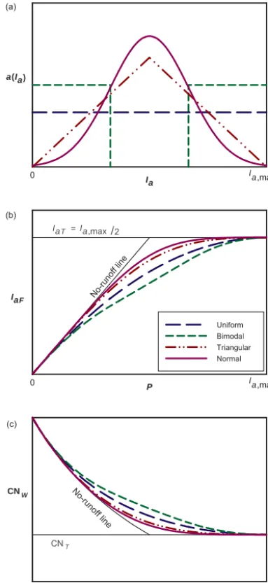
2.5 IaFand CNWcurves for various distributions ofIa The functional form ofa(Ia)defines the areal distribution
ofIawithin a watershed. We considered idealized functional
forms ofa(Ia)that correspond to uniform, normal,
triangu-lar, and bimodal distributions (Table 1). In eacha(Ia), the
maximum or other key value was constrained so that the to-tal area under the distribution was unity. For example, they coordinate of the apex in the triangular distribution must be equal to 2/Ia,max(Table 1). In the case of normal distribution,
however, the area under the curve is unity only when the lim-its are infinite. Therefore, a standard deviation (σ) much less thanIa,maxwas used so that the area under the curve within
the range 0≤Ia≤Ia,maxis approximately equal to unity.
For each distribution, the corresponding functional form ofIaFwas determined using Eq. (16) and the results are
pre-sented in Table 1. For the general case ofa(Ia)as a
poly-nomial, the correspondingIaF is a polynomial two degrees
higher thana(Ia). For the normal distribution,IaFis a
com-bination of Gaussian and error functions (Table 1).
For the purpose of comparison, symmetrical versions of the distributions were considered such that all of them have the same minimum, mean, and maximum values ofIa
(Fig. 8a). The minimum value ofIawas set to zero and the
maximum value wasIa,max. Therefore, the mean for all the
distributions wasIa,max/2.
The kurtosis (peakedness) ofa(Ia)has a major influence
on the shapes of IaF and CNW plotted as functions of P
P IaF
Uniform Bimodal Triangular Normal
P
CNW
Ia a(Ia)
Ia,max 0
IaT = Ia,max/2
No-runoff line
CNT No-runoff line (a)
(b)
(c)
Ia,max 0
I a,max 0
Figure 8. (a)Various symmetrical distributions ofIawith the same minimum (zero), mean (Ia,max/2), and maximum (Ia,max);(b)the correspondingIaF curves calculated using Eq. (16);(c)the corre-sponding CNWcurves calculated using Eq. (10).
whereas the bimodal distribution has the least. As the kurto-sis decreases, theIaF and CNWcurves deviate further from
the bounding lines (Fig. 8). When there is a gap in the distri-bution, as in the case of the bimodal distridistri-bution, the corre-spondingIaF curve is linear for the range spanning the gap.
This is consistent with the discrete case whereIaFwas
repre-sented by line segments for the gaps in between the discrete values ofIai (Fig. 4).
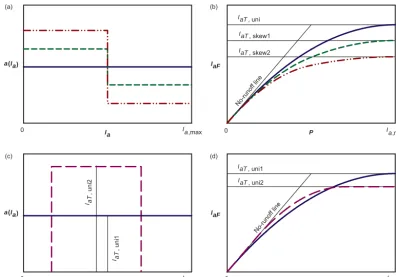
Skewness ofa(Ia)also affectsIaF, and this is illustrated
by an idealized case where an initially uniform distribution is positively skewed (Fig. 9a and b). The mean of a(Ia),
which is equal toIaT(Eq. 17), decreases with increasing
pos-itive skewness. This is important because a land use change such as conversion of forest to urban land is expected to in-crease the positive skewness (i.e., more low values of Ia).
During the conversion,Ia,maxremains unchanged while some
forested land remains. When the entire forest is converted, Ia,maxdrops to a lower value.
The analysis also shows that a watershed cannot be char-acterized or compared with other watersheds using a single value of CN (such as CN∞used in asymptotic fitting, Eq. 7).
Depending on the distribution of heterogeneity, the relative runoff potential of a watershed can beP dependent. This is illustrated by considering two uniform distributions, uni1 and uni2, where uni2 has a narrower range and a smaller mean than uni1 (Fig. 9c). For smaller values ofP,IaF,uni1< IaF,uni2 (Fig. 9d) and therefore CNW,uni1>CNW,uni2. However, for larger values ofP, the converse is true. Thus, the watershed with uni1 generates more runoff for smaller values of P, whereas the watershed with uni2 generates more runoff for larger values ofP.
3 Effect of heterogeneity onS
Similar to the case ofIa, the presence of heterogeneity also
causes the effectiveS of a watershed (SW) to vary with P.
The functional form ofSW depends not only on the
poten-tial maximum retentions of the HRUs (values ofSi) but also on the values of Iai.SW can be estimated using Eq. (2) if
the quantitiesIaW, QW, and FW are known. A distributed
modeling approach can be used to calculate these quanti-ties for a heterogeneous watershed. Distributed CN models, e.g., SWAT (Gassman et al., 2007), commonly calculateQW
as the area-weighted average ofQis, and this assumption can also be extended toFW. Thus,
QW=
n X
i=0
aiQi,
FW=
n X
i=0
aiFi. (21)
Using Eq. (21) and applying mass balance (Eq. 1) at water-shed and HRU scales gives Eq. (14) forIaW. This shows that
IaWcalculated using a distributed model is equal toIaF.
Writing an expression forSW in terms ofIai andSi val-ues for a general case of a heterogeneous watershed is cum-bersome. Therefore, it is only presented graphically for an example of a heterogeneous watershed. However, an expres-sion forSWcan be presented in a compact form for a special
case where all the values ofIai are zero as ifIai=0∀i∈ {0,1, . . .n}
SW=
n P
i=0
aiSi
P+Si
n P
i=0
ai
P+Si
[image:9.612.67.259.81.498.2]Ia a(Ia)
P IaF
IaT, uni1
No-runoff line
IaT, uni2
Ia a(Ia)
Ia,max
0 P
IaF
IaT, uni
No-runoff line
IaT, skew1
IaT, skew2
(a)
(c)
Ia,max 0
Ia,max 0
Ia,max 0
(b)
(d)
I aT
, uni2
I aT
[image:10.612.99.496.78.355.2], uni1
Figure 9.Effect of skewness, mean, and range ofa(Ia)on IaF (a)uniform, uni (solid), and two positively skewed distributions, skew1 (dashed) and skew2 (dash, dot, dot);(b)IaFas a function ofP for the distributions shown in(a);(c)uniform distributions uni1 (solid) and uni2 (dashed) where uni2 has a narrower range of values ofIaand a smaller mean than uni1;(d)IaFas a function ofP for the distributions shown in(c).
Thus, SW varies from the area-weighted harmonic mean n
P
i=0
ai
Si
−1
when P=0 to the area-weighted arithmetic mean
n P
i=0
aiSi
whenPS.
To illustrate the effect of heterogeneity onSW, an example
watershed with the storage distribution shown in Table 2 was considered. The variation ofSWwithP was analyzed for the
cases ofλi=0 andλi=0.2 (Fig. 10). In both cases,SW
in-creases withP and approaches the area-weighted arithmetic mean, S∞, for large values ofP. In the case ofλi=0, the slope of the curve is maximum at the origin and decreases monotonically withP. In the case ofλi=0.2, however, the slope is zero at the origin and generally increases with P untilP≈Ian=40 mm (P≈Ia,maxfor the continuous case),
where it reaches its maximum value. Thereafter the slope de-creases monotonically withP, giving anS-shaped curve. In other words, the slope generally increases withP until the entire watershed area contributes to the runoff and decreases thereafter.
The similarities between IaW andSW are that they both
increase withP and have an upper limit equal to the area-weighted arithmetic mean of their respective components.
The difference is thatIaWreaches its upper limit ofIaT for
a finite value ofP (P =Ian orP=Ia,max), whereasSW
re-quires large values ofP (PS) to reach its upper limit of S∞. Moreover,SWvs.P is an S-shaped curve whenλi>0.
This shows thatIaWandSWare not proportional, i.e.,λWis
not a constant even thoughλivalues are assumed to be equal and constant.
4 Application
The analysis from previous sections shows thatIaWandSW
are functions ofP and gives their functional forms. Incorpo-rating these functions in the lumped-parameter application can potentially improve the performance of the CN method. 4.1 IaWas a function ofP
The distributed parameter modeling approach, Eq. (21) with the application of mass balance (Eq. 1) at watershed and HRU scales, shows thatIaW=IaF.IaF is given by Eq. (14)
for the discrete case and Eq. (16) for the continuous case. All the distributions in Table 1, except the normal distribution, gave a zero-intercept polynomial forIaF. Therefore, using a
Table 1.Functional forms ofa(Ia)andIaFfor various synthetic distributions.
Distribution Graph a(Ia) IaF
Uniform
Ia a(Ia)
Ia,max 0
max 1
a, I
1
Ia,max P−
P2
2Ia,max
Normal
Ia a(Ia)
Ia,max 0
1
σ
√
2πe
−(Ia−µ)2/(2σ2) P−√σ
2π
h
e−(P−µ)2/(2σ2)−e−µ2/(2σ2)i
−(P−µ)
2 h
erfP√−µ
2σ
+erfõ
2σ
i
Triangular
Ia a(Ia)
Ia,max 0
a, a,
I max
2
a
2Ia
aIa,maxifIa≤a P− P3
3aIa,max ifP≤a 2
(Ia,max−a)
1− Ia Ia,max
ifa < Ia 1
(Ia,max−a)
h −a2
3 +Ia,maxP−P2+
P3 3Ia,max
i
ifa < P
Bimodal
b
a Ia
a(Ia)
Ia,max 0
a, - au v =
I max- b 1
u
v
uifIa≤a P−uP
2 2 ifP≤a
0 ifa < Ia< b ua
2
2 +(1−ua)P ifa < P < b
vifb≤Ia ua
2−vb2
2 +(1−ua+vb)P−
[image:11.612.65.269.534.682.2]vP2 2 ifb≤P
Figure 10.Variation ofSWwithP in a heterogeneous watershed with the storage distribution shown in Table 2.
IaW=c1P−c2P2∀P ≤Ia,max
IaW=IaT=c1 Ia,max−c2 Ia,max2∀P > Ia,max (23)
is an efficient way to describeIaW. In Eq. (23),c1andc2are
calibration parameters such that 0≤c1≤1 andc2≥0. Since
the slope ofIaWis zero atP=Ia,max(Eq. 19), it follows from
Eq. (23) that Ia,max=
c1
2c2
,
IaT=
c21 4c2
. (24)
Similarly, the slope ofIaWis unity atP=0 soc1should be
allow for the approximation of piecewise functions (e.g.,IaF
for triangular and bimodal distributions in Table 1). More-over, the analysis for the discrete case shows that when HRUs with zero initial abstraction are present, the origin is a kink point where the slope abruptly jumps from unity to 1−a0.
To avoid over-parameterization of the model, a polynomial of degree>2 forIaWwas not considered.
4.2 SWas a function ofP
The sigmoid-shaped function ofSW, with the conditions that
SW=0 whenP=0 and that the maximum slope occurs at
P =Ia,max, requires at least two parameters to describe it.
However, this along with Eq. (23) would also increase the number of calibrated parameters in the CN method, increas-ing its complexity and potentially causincreas-ing non-uniqueness. A relatively simple approach is to assume thatSWis constant
similar to the conventional CN method. Another approach is to assume thatSWis proportional toIaW; i.e., Eq. (3) is
ap-plicable for a heterogeneous watershed.
Here the emphasis is placed on treatingIaWas a function
of P while offering some flexibility on how SWis treated.
This is because the variation of IaW with P had a
signifi-cant impact on the model performance, whereas including the variation ofSWwithP showed only marginal or no
im-provement. This may be becauseIaWis a component of mass
balance (Eq. 1) whileSWis not.FW, which is the filled
por-tion ofSW, is a component of mass balance and varies withP
even ifSWis assumed to be a constant. Therefore, to
main-tain the simplicity of the CN method and avoid the problems of over-parameterization and non-uniqueness, modeling the sigmoid-shaped function ofSWis omitted.
4.3 Lumped-parameter models
Lumped-parameter application of the CN method was modi-fied by treatingIaWas a function ofPas described in the
pre-vious section. Modified lumped-parameter CN models were evaluated by comparing their performance with that of the conventional lumped-parameter CN models.
4.3.1 Conventional models (CMs)
Conventional CN models are defined by Eqs. (1) through (5) and by the assumption thatIaWandSWare independent ofP.
In this study two types of conventional models, referred to as CM0.2 and CMλ, were used. In CM0.2, λW was fixed
at 0.2, and, in CMλ,λWwas determined by calibration. Thus,
CM0.2 had one free parameter,SW, whereas CMλhad two
free parameters,λWandSW.
4.3.2 Variable initial abstraction models (VIMs) VIMs are defined by Eqs. (1), (2), (4), (5), and (23), and they have three free parameters. IfSWis assumed to be
[image:12.612.379.476.95.175.2]indepen-dent ofP, then the model requires calibration ofc1,c2, and
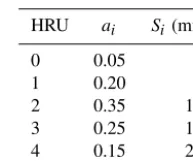
Table 2.Storage distribution in a hypothetical heterogeneous wa-tershed used to illustrate the variation ofSWwithP.
HRU ai Si(mm)
0 0.05 0
1 0.20 50
2 0.35 100
3 0.25 150
4 0.15 200
SWand is referred to as VIMS. If Eq. (3) is also included,
then the model requires calibration ofc1,c2, andλWand is
referred to as VIMλ.
5 Evaluation
Lumped-parameter models described in the previous section were evaluated in their ability to predict runoff and account for watershed heterogeneity. Accounting for heterogeneity means that the model accurately predictsIaWandSW, as well
as runoff from smaller events. This is because (i)IaWandSW
as functions ofP are directly related to heterogeneity, and (ii) the model’s inability to account for their variation withP causes underestimation of runoff in smaller events.
Evaluation of lumped-parameter models requires the data forIaW,QW, andSW. This is generated using a distributed
parameter model application of the CN method. The assump-tion is that a distributed parameter model accounts for hetero-geneity, and therefore its estimates ofIaW,QW, andSWare
accurate.
5.1 Distributed parameter model
In a distributed parameter model, Eqs. (1) through (5) are applicable at the HRU scale, with the assumption thatIai and Si are independent ofP. OnceQi andFi are calculated for each HRU, watershed-scale quantitiesIaW,QW,FW, andSW
are calculated using Eqs. (14), (21), and (2).
The distributed parameter model was applied to an ideal-ized synthetic watershed with the storage distribution shown in Table 2, for the cases ofλi=0, 0.2, and 0.5. A range of values ofP were synthetically generated such that they vary lognormally from 0.1 to 200 mm with a median of 8 mm. For each rainfall event,IaW,QW,FW, and SWwere calculated
5.2 Model evaluation criteria
Each lumped-parameter model was calibrated by minimiz-ing the sum of the squared residuals between its predicted runoff (QW) and the baseline from the distributed
parame-ter model. All the models were evaluated using the Nash– Sutcliffe efficiency parameter (NSE), the standard error of estimate (SEE), and the percent bias (PB) (McCuen, 2003; Moriasi et al., 2007). NSE can vary from−∞to 1. The cal-culations and observations are exactly equal when NSE=1. The calculations are only as good as the average observa-tion when NSE=0. SEE is the root-mean-square residual ad-justed to the degrees of freedom (Santikari, 2017). A smaller SEE indicates a better performance, and its ideal value is zero. PB indicates whether the model is over- (PB<0) or under-predicting (PB>0) on average. The optimal value for PB is zero.
NSE values were calculated for the model predictions of runoff (NSEQ), initial abstraction (NSEIa), potential
max-imum retention (NSES), and runoff from events with P
less than the median value (NSEQ50). Relative NSE, rNSE (Krause et al., 2005), was used instead of NSE when the lat-ter was strongly influenced by larger events. PB values were calculated for runoff from all the events (PBQ) and runoff from events withP less than the median value (PBQ50). SEE was calculated for runoff from all the events (SEEQ).
NSEIa and NSES indicate how accurately a
lumped-parameter model predicts the watershed heterogeneity. NSEQ, SEEQ, and PBQ reflect the overall accuracy in a model prediction of runoff from all the events, whereas NSEQ50 and PBQ50 reflect the accuracy in predicting runoff from smaller events (P <8 mm). Conventional models tend to under-predict runoffs from smaller events because of the usage of constant IaandS. They often falsely predict
zero-runoffs because the runoff condition (P > Ia) cannot be
over-come in smaller events. NSEQ50 and PBQ50 are used to ex-pose this shortcoming.
6 Results and discussion
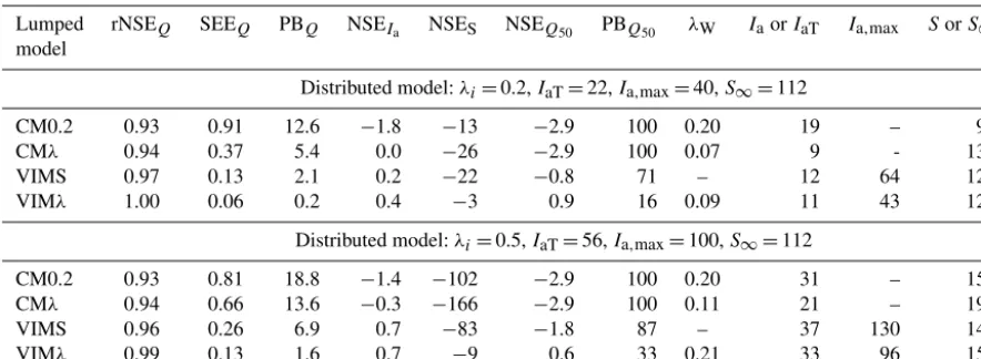
The results show that using variable initial abstraction im-proved the accuracy of model predictions of runoff and het-erogeneity (Table 3). Based on their overall performance, the models can be arranged from the best to the worst as VIMλ >VIMS>CMλ >CM0.2. Results for the case of λi=0 are not presented in Table 3 because VIMλ, VIMS, and CMλperformed equally well while CM0.2 was the worst (i.e., VIMλ=VIMS=CMλ >CM0.2).
Variable Ia models predicted runoff better than the
con-ventional models. It was not possible to determine relative model performance using NSEQ because it was 1.0 for all the models. This was because NSEQwas strongly influenced by a few larger events, and a good fit in these events was suf-ficient to render NSEQ=1.0. Therefore, rNSEQ(Krause et
al., 2005) was calculated instead and listed in Table 3. Larger events had greater influence on rNSEQas well, but the val-ues varied slightly between the models (Table 3). rNSEQ in-creased down the table whereas SEEQdecreased, with both indicating an improvement in model performance. PBQwas positive for all the models, indicating that they all under-predicted runoff. The extent of under-prediction, however, was smaller in variableIamodels than the conventional
mod-els.
Variable Ia models gave a better estimate of watershed
heterogeneity than the conventional models as indicated by the higher values of NSEIa and NSES(Table 3). NSEIa was zero or negative in the conventional models, whereas it varied from 0.2 to 0.7 in the variableIamodels. NSESwas negative
in all the models, indicating that their estimates ofS were poor. In the case of the conventional models this was due to using uniformIa andS and thereby homogenizing the
wa-tershed. In the case of the variableIa models, this was due
to their inability to model theS-shaped function ofS. Based on NSEIaand NSES, VIMλwas the best model in estimating watershed heterogeneity.
VariableIa models also predicted runoff better than the
conventional models in smaller rainfall events (P <8 mm) as indicated by NSEQ50and PBQ50. In both cases ofλi=0.2 and 0.5, only HRU no. 0 (Table 2) produced runoff when P <8 mm. This was similar to the case of a partial source area. As CM0.2 and CMλpredicted an Ia>8 mm in both
cases (Table 3), they falsely predicted zero-runoffs in all the events withP <8 mm because the runoff condition (P > Ia)
could not be overcome. Therefore, their PBQ50=100 in both cases, indicating a 100 % under-prediction in small events. Their NSEQ50 was also poor with the same value in both cases. VIMS performed slightly better than the conventional models with 70–90 % under-predictions and with NSEQ50 varying from−0.8 to−1.8 (Table 3). VIMλperformed sig-nificantly better than all the other models with 30 % or less under-predictions and with NSEQ50 varying from 0.6 to 0.9. Even though there were under-predictions, there was no false prediction of zero-runoffs for any of the events in the variable Iamodels.
In the models whereλWwas calibrated (CMλand VIMλ),
it was smaller thanλi (Table 3). This shows that λ at the watershed scale tends to be smaller than that at the HRU scale in the lumped-parameter models. All the models under-predictedIa orIaT with CMλbeing the most severe. There
was also a corresponding over-prediction ofSor S∞by all
the models except for the case ofλi=0.2 in CM0.2. Again, the most over-prediction ofSoccurred in CMλ. The under-prediction ofIa and the corresponding over-prediction ofS
is due to the transfer of storage fromIatoS, which generally
Table 3.The performance of lumped-parameter CN models that were calibrated to the runoff data generated using a distributed CN model for two cases of a synthetic watershed with the storage distribution shown in Table 2. SEE,Ia, andSare in mm. (SEE: standard error of estimate, PB: percent bias, NSE: Nash–Sutcliffe efficiency parameter, rNSE: relative NSE.)
Lumped rNSEQ SEEQ PBQ NSEIa NSES NSEQ50 PBQ50 λW IaorIaT Ia,max SorS∞ model
Distributed model:λi=0.2,IaT=22,Ia,max=40,S∞=112
CM0.2 0.93 0.91 12.6 −1.8 −13 −2.9 100 0.20 19 – 97
CMλ 0.94 0.37 5.4 0.0 −26 −2.9 100 0.07 9 - 132
VIMS 0.97 0.13 2.1 0.2 −22 −0.8 71 – 12 64 121
VIMλ 1.00 0.06 0.2 0.4 −3 0.9 16 0.09 11 43 124
Distributed model:λi=0.5,IaT=56,Ia,max=100,S∞=112
CM0.2 0.93 0.81 18.8 −1.4 −102 −2.9 100 0.20 31 – 155
CMλ 0.94 0.66 13.6 −0.3 −166 −2.9 100 0.11 21 – 197
VIMS 0.96 0.26 6.9 0.7 −83 −1.8 87 – 37 130 140
VIMλ 0.99 0.13 1.6 0.7 −9 0.6 33 0.21 33 96 153
6.1 Storage transfer fromIatoS
The storage in a watershed is distributed betweenIaandS.Ia
is the part of the storage that does not produce runoff while being filled, whereasSis the part that produces runoff while being filled. Using Eqs. (2) and (1) it can be shown that S=(P−Ia) (P−Ia−Q)
Q . (25)
For an observed storm event,P andQare known and there-fore are constants in Eq. (25), so decreasing Ia will
in-crease S. However, the magnitude of increase in S will be greater than the magnitude of decrease in Ia. This is
illus-trated by differentiating Eq. (25) and using Eq. (4) to give dS
dIa = −
1+ 2S
P−Ia
∀P > Ia. (26)
Thus, dS/dIais always negative and less than or equal to−1.
If (P−Ia)S or S≈0, then dS/dIa≈ −1, implying an
equal transfer in storage between Ia and S. However, as
P decreases, dS/dIa becomes less than −1, implying that
S changes more rapidly than Ia. In other words, the
rela-tive change of magnitude in S with respect to Ia is large
for smallerP, decreases with increasingP, and approaches unity for large values ofP.
Storage transfer is evident when the values of Ia andS
for the models CM0.2 and CMλ are compared (Table 3). For the case ofλi=0.2,Iadecreased from 19 mm in CM0.2
to 9 mm in CMλ, whereasS increased from 97 to 132 mm, i.e., dS/dIa= −3.5. Similarly, for the case of λi=0.5, dS/dIa= −4.2.
A transfer of storage from Ia to S improves the
perfor-mance in the conventional models (i.e., CMλ >CM0.2) be-cause (i) a smallerIa reduces the percentage of events with
falsely predicted zero-runoffs and (ii) it allows the model to
mimic a variableIa. Because of a largerIa, CM0.2 falsely
predicted zero-runoffs in 80 % of the events forλi=0.2 and in 85 % of the events forλi=0.5. In the case of CMλ, the percent of events with zero-runoffs dropped to 57 % and 81 %, respectively, because Ia for CMλ was smaller than
CM0.2. Mimicking variableIacan be explained by
consid-eringIaF andF, which are the filled portions ofIa andS,
respectively.IaF andF have similar functional relationships
withP (compare Fig. 6 to Fig. 1); i.e., they both increase with P and approach a constant for large values ofP. In the con-ventional CN models, there is no provision to representIaF
as a function ofP. However,F is understood to be a function ofP and is treated as such through Eq. (2) and Fig. 1. There-fore, by transferring the storage fromIa toS, CMλusesF
as a surrogate forIaF, thereby partly mimicking the variable
nature ofIaF.
Storage transfer fromIatoSalso causes a decrease inλW
(Table 3). Conversely, whenλWdecreases, storage is
trans-ferred fromIatoS. This is important because several studies
(Baltas et al., 2007; D’Asaro and Grillone, 2012; Shi et al., 2009; Woodward et al., 2003) found that the optimal value of λWwas much less than 0.2 and even close to zero in many
watersheds. This shows that there is a positive correlation be-tween a decrease inλW, storage transfer fromIatoS, and a
general increase in model performance for the reasons men-tioned above.
6.2 Application to real watersheds
wa-Table 4. Performance of the models for the cases of λi=0.2 and 0.5, when the degree of heterogeneity in the synthetic watershed (Table 2) was increased by doubling the values ofSi for HRUs 3 and 4.
Lumped λi=0.2 λi=0.5
model rNSEQ SEEQ rNSEQ SEEQ
CM0.2 0.92 1.54 0.92 1.30
CMλ 0.95 0.19 0.94 0.38
VIMS 0.97 0.12 0.96 0.25
VIMλ 1.00 0.06 1.00 0.12
tersheds. Between VIMλ and CM0.2, 1NSEQ<0.05 in one watershed, 0.05≤1NSEQ<0.7 in six watersheds, and 1NSEQ≥0.7 in two watersheds. Between VIMλand CMλ, 1NSEQ<0.05 in three watersheds, 0.05≤1NSEQ<0.1 in four watersheds, and 1NSEQ≥0.1 in two watersheds. Based on their performance, the models can be arranged from the best to the worst as VIMλ >VIMS>CMλ >CM0.2, which is consistent with results from their application to the synthetic watershed.
6.3 Effect of degree of heterogeneity
The degree of heterogeneity, defined as the sharpness of change in CN, Ia, orS between the HRUs, may affect the
relative performance of the models. To verify this, the de-gree of heterogeneity of the synthetic watershed (Table 2) was increased by doubling the values of Si for HRUs 3 and 4 while the others were left unchanged; i.e., the modi-fied distribution wasS0=0 mm,S1=50 mm,S2=100 mm,
S3=300 mm, andS4=400 mm. The models were applied to
this modified synthetic watershed, for the cases ofλi=0.2 and 0.5, and their performances were assessed using rNSEQ and SEEQ.
Comparing the results (Tables 3 and 4) shows that the performance of VIMs remained nearly the same, whereas the performance of CM0.2 decreased and that of CMλ in-creased. The relative order of performance remained un-changed, i.e., VIMλ >VIMS>CMλ >CM0.2.
The results from real watersheds (Santikari, 2017; San-tikari and Murdoch, 2018) also show that the performance of CM0.2 was poor, NSEQ<0.25, in watersheds with a sharp change in CN. Therefore, CM0.2 is unsuitable when the degree of heterogeneity is large. CMλperformed mod-erately well on synthetic and real watersheds with a large degree of heterogeneity, possibly by transferring the storage (Sect. 6.1). So, CMλis suitable for predicting overall runoff, but unreliable for predicting heterogeneity or runoff from small events. VIMs outperformed CMλin synthetic (Table 4) as well as real watersheds (Santikari, 2017; Santikari and Murdoch, 2018) with a large degree of heterogeneity, and therefore they are more reliable.
6.4 Model suitability
One of the main objectives of this study was to improve the predictive ability of the CN method while maintain-ing its simplicity. Usmaintain-ing the number of calibrated param-eters as an indicator, the models can be arranged in the order of increasing complexity as CM0.2 (one)<CMλ (two)<VIMS=VIMλ(three). CM0.2 was the simplest but also had the poorest performance (Tables 3 and 4). Moreover, there is no justification in fixingλWat 0.2 or any other
con-stant as its optimal value can vary from zero to one (Hawkins et al., 2008). Therefore, the usage of CM0.2 is not recom-mended.
CMλ predicted the overall runoff and the runoff from small events better than CM0.2. Often, the optimalλW is
much smaller than 0.2 and this allows CMλto partly mimic a variableIaFby transferring storage fromIatoS. A smaller
λWalso reduces the false prediction of zero-runoffs, which
are completely eliminated when λW=0. Compared to the
variableIa models, CMλ is a poor predictor of runoff and
watershed heterogeneity (Table 3). However, in watersheds with negligibleIai values (orλi≈0) CMλ can perform as well as the variableIamodels and therefore may be
prefer-able because of its simplicity.
VariableIamodels show that significant improvement in
the model prediction of overall runoff and heterogeneity can be achieved by using one extra parameter (Table 3). This is because the functional form ofIaF(Eq. 23) is consistent with
the observations (Fig. 2c and d) and the results from the theo-retical analysis of heterogeneous watersheds (Eq. 16, Fig. 6, and Table 1). Using variableIaalso improved the runoff
pre-dictions in small events and eliminated the false prediction of zero-runoffs. Therefore, their application is recommended in heterogeneous watersheds with nonzero initial abstractions.
When the watershed heterogeneity is known in great de-tail such that the number of calibrated parameters≤3, a dis-tributed modeling approach (e.g., SWAT; Gassman et al., 2007 or Soulis and Valianzas, 2013) may be preferable over the variableIa models. A distributed parameter model has
advantages similar to the variableIamodels over the
conven-tional models. It would inherently account for the variation of the CN method’s parameters spatially and withP. It would also avoid the false prediction of zero-runoffs in small events because HRUs with larger CNs, which generate runoff even in small events, are explicitly considered. When the hetero-geneity is unknown, however, the number of calibrated pa-rameters (for values of CNi andai) in a distributed model withnHRUs is 2n−1. This number would increase further if values ofλi are also calibrated. Therefore, when the num-ber of calibrated parameters>3, application of a variableIa
[image:15.612.66.268.117.199.2]6.5 Model limitation
A strength of the models proposed in this paper is that they provide a compact way to account for the spatial variation of CN,Ia, orS(watershed heterogeneity), but a limitation is that
they do not account for the temporal variation. During dry pe-riods,IaandS increase whereas, CN decreases. The
behav-ior is opposite during the wet periods. Changes in land cover introduce additional temporal variations. Therefore, the cal-ibrated model parameters in this paper can be considered as temporal averages. The models may underpredict runoff dur-ing wet periods and overpredict durdur-ing dry periods. A pro-cedure to account for temporal variations using antecedent moisture is described by Santikari (2017) and Santikari and Murdoch (2018).
Another limitation of VIMs is that the CN values calcu-lated using Eqs. (5) or (10) are incompatible with the stan-dard CN values (NRCS, 2003; USDA, 1986) derived using CM0.2. However, this limitation is not unique to VIMs be-cause any method, including CMλ, which involves an al-tered relationship between Ia andS (i.e.,λ6=0.2) leads to
CN values that are incompatible with those derived from CM0.2. Given that (i) CM0.2 is a poor predictor of runoff (Tables 3 and 4; Santikari, 2017; Santikari and Murdoch, 2018) and (ii) the evidence contradictsλ=0.2 (Baltas et al., 2007; D’Asaro and Grillone, 2012; Shi et al., 2009; Wood-ward et al., 2003), the above-mentioned limitation is an ac-ceptable compromise.
7 Conclusions
Watershed heterogeneity causes calculated values of Ia,S,
and CN to vary with P. Therefore, using a single effective value of these quantities at the watershed scale can lead to systematic errors in the predictions ofQ. This problem can be mitigated by treatingIa,S, or CN as functions of P. A
theoretical analysis assuming spatial variation ofIaled to the
following conclusions.
1. EffectiveIaof a watershed is equal to the filled portion
of the total storage inIa. The total storage (calledIaT)
is constant, whereas the filled portion (calledIaF)is a
function ofP (Eq. 16). Variation ofIaFwithP (Fig. 6)
is similar to the variation of calculated Ia (also called
effectiveIaorIaW) withP (Fig. 2c and d). This shows
thatIaW=IaF, which is also supported by a distributed
model using many HRUs (Eq. 21). The form ofIaFas
a function ofP depends on the spatial distribution ofIa
within a watershed (Table 1, Figs. 8 and 9).
2. λdecreases with increasing spatial scale. Using CNW,
calculated as the area-weighted average of CNi values (CNs of the HRUs), and the definition ofIa, it can be
shown thatλW< λi(Eqs. 8 through 11). Even whenλW
was calibrated using CMλ, the result wasλW< λi (Ta-ble 3). This shows that in conventional modelsλat the watershed scale tends to be smaller than that at the HRU scale; i.e.,λdecreases with increasing spatial scale. 3. Replacing Ia with IaF can account for heterogeneity.
Heterogeneity causes the effectiveIaof a watershed to
vary with P, so to account for heterogeneity variable Iamodels (VIMs) replaceIawithIaF, which is a
func-tion of P (Fig. 6). For practical purposes,IaF can be
treated as a quadratic function ofP (Eq. 23) with two free parametersc1andc2that need to be calibrated. In
addition, the model also requires the calibration of ei-therS(VIMS) orλ(VIMλ).
4. VariableIamodels perform better than the conventional
models. VariableIa models predict runoff and
hetero-geneity better than the conventional models CM0.2 (λ=0.2) and CMλ(calibratedλ). They also eliminate the false prediction of zero-runoffs and improve runoff predictions in small events. Based on their overall per-formance, the models are arranged from the best to the worst as VIMλ >VIMS>CMλ >CM0.2.
5. Storage transfer can improve model performance. Stor-age transfer fromIatoSgenerally improves the model
performance because the filled portions of Ia and S,
IaFandF, respectively, have similar functional
relation-ships withP (compare Figs. 6 to 1). This enables a CN model to partly mimic a variableIaF by usingF as its
surrogate. Storage transfer also lowers the thresholdP for runoff generation, thereby reducing the false pre-diction of zero-runoffs. Storage transfer decreasesλW
(Eq. 3), and this can explain why the optimal value of λWfrom published studies is much less than 0.2 or even
zero in many watersheds.
Appendix A: List of symbols
ai fractional area of theith HRU
a(Ia) probability density function of areal occurrence ofIa
CM0.2 conventional curve number model withλ=0.2 CMλ conventional curve number model with calibratedλ CN curve number, applicable to any spatial scale CNi curve number of theith HRU
CNT curve number of a watershed whenIaF=IaT
CNW curve number of a watershed
F cumulative infiltration after runoff begins HRU hydrologic response unit
Ia initial abstraction, applicable to any spatial scale
IaF areal average of the filled portion ofIaT
Iai initial abstraction of theith HRU
IaT areal average of the total initial abstraction
IaW effective initial abstraction of a watershed
Ia,max maximum value ofIawithin a watershed
λ initial abstraction ratio, applicable to any spatial scale λi initial abstraction ratio at HRU scale
λW initial abstraction ratio at watershed scale
m number of fully filled HRUs in whichIai6=0 n number of HRUs in whichIai6=0
NSE Nash–Sutcliffe efficiency parameter P event rainfall
PB percent bias Q event runoff
R2 coefficient of determination
S potential maximum retention, applicable to any spatial scale Si potential maximum retention ofith HRU
S∞ maximum value ofSW, which occurs whenP is infinitely large
SW effective potential maximum retention of a watershed
SEE standard error of estimate
Author contributions. VS conceived the idea and performed the analysis. LM supervised the analysis and influenced the overall di-rection and content of the work. Both VS and LM wrote the paper.
Competing interests. The authors declare that they have no conflict of interest.
Acknowledgements. Primary funding for this study was provided by the USDA Natural Resources Conservation Service (NRCS-69-4639-1-0010) through the Changing Land Use and Environ-ment (CLUE) project at Clemson University. Additional support was provided by the USDA Cooperative State Research, Education, and Extension Service under project number SC-1700278.
Edited by: Thomas Kjeldsen
Reviewed by: two anonymous referees
References
Baltas, E. A., Dervos, N. A., and Mimikou, M. A.: Technical note: Determination of the SCS initial abstraction ratio in an experi-mental watershed in Greece, Hydrol. Earth Syst. Sci., 11, 1825– 1829, https://doi.org/10.5194/hess-11-1825-2007, 2007. Bingner, R. L., Theurer, F. D., and Yuan, Y.: AnnAGNPS technical
processes documentation 5.2, 2011.
D’Asaro, F. and Grillone, G.: Empirical investiga-tion of Curve Number Method parameters in the Mediterranean area, J. Hydrol. Eng., 17, 1141–1152, https://doi.org/10.1061/(ASCE)HE.1943-5584.0000570, 2012. D’Asaro, F. and Grillone, G.: Discussion: “Curve Number
deriva-tion for watersheds draining two headwater streams in lower coastal plain South Carolina, USA” by Epps T. H., Hitchcock D. R., Jayakaran A. D., Loflin D. R., Williams T. H., and Amatya D. M., J. Am. Water Resour. Assoc., 51, 573–578, https://doi.org/10.1111/jawr.12264, 2015.
Gassman, P. W., Reyes, M. R., Green, C. H., and Arnold, J. G.: The Soil and Water Assessment Tool – Historical development ap-plications, and future research directions, T. ASABE, 50, 1211– 1240, 2007.
Hawkins, R.: Asymptotic determination of runoff Curve Numbers from data, J. Irrig. Drain. Eng., 119, 334–345, https://doi.org/10.1061/(ASCE)0733-9437(1993)119:2(334), 1993.
Hawkins, R., Ward, T., Woodward, D., and Van Mullem, J.: Curve Number hydrology: State of practice, American Society of Civil Engineers, Reston, VA, 2008.
Hjelmfelt Jr., A. T., Woodward, D. A., Conaway, G., Plummer, A., Quan, Q. D., Van Mullen, J., Hawkins, R. H., and Ri-etz, D.: Curve numbers, recent developments, in: Proc. of the 29th Congress of the Int. As. for Hydraul. Res., 17–21 Septem-ber 2001, Beijing, China, 2001.
HydroCAD: http://www.hydrocad.net, last access: August 2018. Kent, K. M.: A method for estimating volume and rate of runoff in
small watersheds, Technical Paper 149, USDA SCS, Washing-ton, D.C., 1968.
Knisel, W. G. and Douglas-Mankin, K. R.: CREAMS/GLEAMS: Model use, calibration, and validation, T. ASABE, 55, 1291– 1302, 2012.
Krause, P., Boyle, D. P., and Bäse, F.: Comparison of different effi-ciency criteria for hydrological model assessment, Adv. Geosci., 5, 89–97, https://doi.org/10.5194/adgeo-5-89-2005, 2005. McCuen, R. H.: Modeling hydrologic change: Statistical methods,
Lewis Publishers, Boca Raton, Florida, 2003.
Mishra, S. K., Sahu, R. K., Eldho, T. I., and Jain, M. K.: An improved Ia–S relation incorporating antecedent moisture in SCS-CN methodolog, Water Resour. Manage., 20, 643-660, https://doi.org/10.1007/s11269-005-9000-4, 2006.
Moriasi, D. N., Arnold, J. G., Van Liew, M., Bingner, R. L., Harmel, R. D., and Veith, T. L.: Model evaluation guidelines for sys-tematic quantification of accuracy in watershed simulations, T. ASABE, 50, 885–900, 2007.
Neitsch, S. L., Arnold, J. G., Kiniry, J. R., and Williams, J. R.: Soil and Water Assessment Tool theoretical documentation (ver-sion 2005), Agricultural Research Service, Temple, TX, 2005. NRCS: National engineering handbook: Part 630, Hydrology,
USDA, Washington, D.C., 2003
Panday, S. and Huyakorn, P. S.: A fully coupled physically-based spatially-distributed model for evaluating sur-face/subsurface flow, Adv. Water Resour., 27, 361–382, https://doi.org/10.1016/j.advwatres.2004.02.016, 2004. Ponce, V. and Hawkins, R.: Runoff Curve Number:
Has it reached maturity?, J. Hydrol. Eng., 1, 11–19, https://doi.org/10.1061/(ASCE)1084-0699(1996)1:1(11), 1996. Rallison, R. E. and Miller, N.: Past, present, and future SCS
runoff procedure, in: Proceedings of the international symposium on rainfall runoff modeling: Rainfall–runoff relationship, 18– 21 May 1981, Mississippi State University, Mississippi, edited by: Singh, V. P., Water Resources Publications, Littleton, Col-orado, 353–364, 1982.
Santikari, V. P.: Accounting for Spatiotemporal Variations of Curve Number using Variable Initial Abstraction and Antecedent Moisture, chap. 5, in: Evaluating Effects of Construction-Related Land Use Change on Streamflow and Water Qual-ity, Doctoral dissertation, https://tigerprints.clemson.edu/all_ dissertations/1942 (last access: August 2018), 2017.
Santikari, V. P. and Murdoch, L. C.: Accounting for spatiotemporal variations of Curve Number using variable initial abstraction and antecedent moisture, in review, 2018.
Shi, Z., Chen, L., Fang, N., Qin, D., and Cai, C.: Research on the SCS-CN initial abstraction ratio using rainfall-runoff event analysis in the Three Gorges Area, China, Catena, 77, 1–7, https://doi.org/10.1016/j.catena.2008.11.006, 2009.
Soil Conservation Service: National engineering handbook: Sec-tion 4, Hydrology, USDA SCS, Washington, D.C., 1956. Soil Conservation Service: National engineering handbook:
Sec-tion 4, Hydrology, chap. 10, USDA SCS, Washington, D.C., 1972.
Soulis, K. X. and Valiantzas, J. D.: SCS-CN parameter determina-tion using rainfall–runoff data in heterogeneous watersheds – the two-CN system approach, Hydrol. Earth Syst. Sci., 16, 1001– 1015, https://doi.org/10.5194/hess-16-1001-2012, 2012. Soulis, K. X., Valiantzas, J. D., Dercas, N. and Londra, P. A.: