www.hydrol-earth-syst-sci.net/18/273/2014/ doi:10.5194/hess-18-273-2014
© Author(s) 2014. CC Attribution 3.0 License.
Hydrology and
Earth System
Sciences
Characterizing hydrologic change through catchment classification
K. A. Sawicz1, C. Kelleher1, T. Wagener1,2, P. Troch3, M. Sivapalan4, and G. Carrillo3
1Department of Civil and Environmental Engineering, The Pennsylvania State University, Pennsylvania, USA 2Department of Civil Engineering, University of Bristol, Bristol, UK
3Department of Hydrology and Water Resources, The University of Arizona, Tucson, Arizona, USA
4Department of Civil and Environmental Engineering and Department of Geography, University of Illinois-Urbana
Champaign, Illinois, USA
Correspondence to: K. A. Sawicz ([email protected])
Received: 30 April 2013 – Published in Hydrol. Earth Syst. Sci. Discuss.: 28 May 2013 Revised: 29 October 2013 – Accepted: 5 December 2013 – Published: 22 January 2014
Abstract. There has been an intensive search in recent years for suitable strategies to organize and classify the very het-erogeneous group of catchments that characterize our land-scape. One strand of this work has focused on testing the value of hydrological signatures derived from widely avail-able hydro-meteorological observations for this catchment classification effort. Here we extend this effort by organiz-ing 314 catchments across the contiguous US into 12 dis-tinct clusters using six signature characteristics for a baseline decade (1948–1958, period 1). We subsequently develop a regression tree and utilize it to classify these catchments for three subsequent decades (periods 2–4). This analysis allows us to assess the movement of catchments between clusters over time, and therefore to assess whether their hydrologic similarity/dissimilarity changes. We find examples in which catchments initially assigned to a single class diverge into multiple classes (e.g., midwestern catchments between peri-ods 1 and 2), but also cases where catchments from different classes would converge into a single class (e.g., midwestern catchments between periods 2 and 3). We attempt to interpret the observed changes for causes of this temporal variability in hydrologic behavior. Generally, the changes in both direc-tions were most strongly controlled by changes in the water balance of catchments characterized by an aridity index close to one. Changes to climate characteristics of catchments – mean annual precipitation, length of cold season or the sea-sonality of precipitation throughout the year – seem to ex-plain most of the observed class transitions between slightly water-limited and slightly energy-limited states. Inadequate
temporal information on other time-varying aspects, such as land use change, limits our ability to further disentangle causes for change.
1 Introduction
where dense observational networks exist, though their in-formation content regarding catchment functions is limited to the decomposition of these observations (Carrillo et al., 2011).
Our own objective is to enable a mapping between climate, physical characteristics and hydrological behavior through classification, while being widely applicable (Wagener et al., 2007). The classification strategy applied in this study was first introduced in Sawicz et al. (2011), who established sim-ilarity between catchments on the basis of hydrologic signa-tures derived from widely available observations of stream-flow, air temperature and precipitation. In the previous study, we used a Bayesian clustering algorithm to understand hy-drologic similarity and dissimilarity across 280 catchments located in the eastern half of the US. Hydrologic similar-ity was defined by proximsimilar-ity in a six-dimensional signature space.
One reason for such a three-dimensional (climate, physical characteristics, hydrologic behavior) mapping is the growing recognition of the increasing nonstationarity of the hydrolog-ical cycle, primarily due to climate and land use change (e.g., Milly et al., 2008). Therefore, incorporating change into a framework for catchment classification is vital to understand and potentially predict future hydrologic response. Land use changes occur due to urbanization (Martin et al., 2012), forest clearance (Andreassian, 2004), and agricultural de-mands/practices (Parton et al., 2005; Mahmood et al., 2006). These changes alter the functional behavior of catchments in terms of how these systems partition, store and release water (Wagener et al., 2007; He et al., 2011). Climate change will increasingly create new boundary conditions in which catch-ments will evolve (Troch et al., 2013). Recent work suggests that climate change can alter the interaction and influence between hydrologic processes within a catchment, and thus behavior of catchments, in intricate ways (e.g., Rosero et al., 2010; Merz et al., 2011). Land use change will potentially have a more immediate impact in many cases, though our predictive ability of its manifestation altered in hydrologi-cal characteristics is still questionable (Wagener, 2007). Any catchment classification system therefore has to account for these changes, or more generally, any classification frame-work should help to inform how and why catchments are changing (Wagener et al., 2010).
In this paper, we combine the concepts of catchment clas-sification and environmental change to investigate in how far a signature-based classification can provide insight into the consequences of and the reasons for the changing behav-ior of catchments over time. To achieve this objective we classify 314 catchments across the US over four consecu-tive decades. We assume that a decade is both required and sufficient to reasonably estimate signature values for classi-fication. Cluster analysis and decision tree models used are based on six different hydrologic signatures. We attempt to (1) identify how catchment classification, and therefore hy-drologic similarity, changes through time and (2) provide
mechanistic explanations for the change identified in our study region.
2 Data and study catchments
The 314 catchments selected for this study are a subset of the MOPEX (Model Parameter Estimation Experiment) database (Duan et al., 2005). Only catchments with at least 95 % data availability across all four selected periods (1948– 1958; 1958–1968; 1968–1978; 1978–1988) were included in the investigation. Catchments that were already heavily im-pacted by human activity during the baseline decade were excluded from the analysis a priori through visual inspec-tion. The spatial density of catchments available through the MOPEX initiative is much higher in the eastern US than in the western US. The MOPEX database includes daily streamflow data from USGS hydro-climatic data net-work, daily precipitation and temperature data from the Nat-ural Resources Conservation Service SNOTEL (snowpack telemetry) and the National Climate Data Center, soil tex-ture data from STATSGO (State Soil Geographic database), and vegetation classification information from the University of Maryland. Further details on the MOPEX data set can be found in our previous study (Sawicz et al., 2011). Other data sets of land cover and watershed characteristics were also used to interpret possible causes of changes in catchment be-havior. Land cover (agriculture, impervious area, forest) data was available from the USDA at 5 yr intervals at the state level (Nickerson et al., 2011). Our analysis also made use of stream network characteristics, geology, number of dams, soil, and topography data collated to USGS stream gages by Falcone et al. (2010).
3 Methods
3.1 Signatures
Six signatures were calculated from long-term records of daily streamflow, air temperature, and precipitation observa-tions per catchment for four decadal periods: (1) 1948–1958 (baseline), (2) 1958–1968, (3) 1968–1978, and (4) 1978– 1988. The hydrologic year was used rather than the calendar year to remove the impacts of carry-over of water storage as snow between calendar years. The US hydrologic year spans from 1 October of a given year to 30 September of the follow-ing year. Signatures were chosen to capture independent in-formation about catchment behavior at annual, seasonal and daily timescales, and to capture average as well as extreme hydrological behavior (Ssegane et al., 2012a, b). For a more detailed discussion of four of these signatures see Sawicz et al. (2011). Two signatures from our previous study, stream-flow elasticity and rising limb density, were replaced with
Q90and normalizedQ10in this study. The reasons for doing
have the least influence on the previous classification result, and secondly, we found it difficult to relate streamflow elas-ticity to other characteristics, which would limit our ability to find mechanistic explanations in this this study. The com-plete list of signatures used in this study is the following.
– Runoff ratio (RQP,[−]), the long-term water balance
represented by the ratio of long-term average stream-flow (Q) to long-term average precipitation (P).
– Baseflow index (BFI,[−]), the portion of streamflow
classified as baseflow, which represents a measure of the volume of water taking longer flow paths through the catchment. In this study we use the one-parameter single-pass digital filter method based on previous studies as reported by Arnold et al. (1995) and Lim et al. (2005).
– Slope of the flow duration curve (SFDC, [−]), the
slope between the 66 % and the 33 % flow ex-ceedance percentiles, which is an indicator of stream-flow variability.
– Ratio of snow days (RSD,[−]), the ratio of
precipita-tion events that occur when mean daily temperature is below 2◦C to the total number of precipitation events. This signature is a proxy for flow seasonality, length of the winter period, and the general significance of snow storage.
– 10th prcentile streamflow (Q10, [−]) is the ratio of
daily streamflow that is exceeded 10 % of the time nor-malized by the mean streamflow. This signature is a measure of high flows.
– 90th percentile streamflow (Q90, [mm]) is purely the
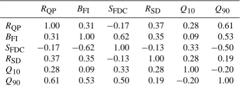
value of daily streamflow that is exceeded 90 % of the time. This signature is a measure of very low flows. One primary requirement for these signatures was that they each provide independent information (Table 1). This was difficult to achieve in case of the flow percentiles and the slope of the flow duration curve. We therefore leftQ90
with-out normalization, while Q10 was normalized, which, as
shown later, had no impact on the regression tree.
3.2 Clustering algorithm
[image:3.595.309.549.93.182.2]The method chosen for this study is a fuzzy partitioning Bayesian mixture-clustering algorithm implemented in the AutoClass C software package (version 3.3.4) (Stutz and Cheeseman, 1995; Cheeseman and Stutz, 1996; Archcar et al., 2009; Kennard et al., 2010). Bayesian mixture modeling is a probabilistic approach in which marginal likelihoods for different classification realizations are estimated and ranked against all other realizations. While a range of different clus-tering algorithms is available, the chosen algorithm has been shown to be effective with respect to its use in environmental
Table 1. Linear correlation values of the six signatures used in this study from the first time period.
RQP BFI SFDC RSD Q10 Q90
RQP 1.00 0.31 −0.17 0.37 0.28 0.61
BFI 0.31 1.00 0.62 0.35 0.09 0.53
SFDC −0.17 −0.62 1.00 −0.13 0.33 −0.50
RSD 0.37 0.35 −0.13 1.00 0.28 0.19
Q10 0.28 0.09 0.33 0.28 1.00 −0.20
Q90 0.61 0.53 0.50 0.19 −0.20 1.00
studies (Reidy Liermann et al., 2011; Kennard et al., 2010; Sawicz et al., 2011). In the AutoClass algorithm, the classi-fication with the highest posterior probability is ultimately chosen as the most likely realization (Webb et al., 2007). Each catchment is assigned to a specific class with a defined probability of membership, which is called the probability of class assignment. A catchment can be assigned to different classes due to the probabilistic nature of the algorithm, and it is only the primary (i.e., highest probability) class assign-ment that is listed. The number of classes is automatically decided during the clustering process. The input variables characterizing the catchments, i.e., the signatures, were log transformed and modeled as normally distributed continu-ous variables with an associated degree of uncertainty. Ad-ditionally, these variables are scaled such that the magnitude differences between signatures do not cause any additional weighting in the calculation of the distance metric.
Due to the probabilistic nature of the AutoClass-C algo-rithm, classification realizations will slightly change over multiple runs. A value of 4 % was assumed to represent the uncertainty in signature values that were used in the Auto-Class run (Sawicz et al., 2011). We used the adjusted Rand index to test the stability of the results across these dif-ferent realizations (ARI, Rand, 1971; Hubert and Arabie, 1985). The ARI takes a value of 0 if the agreement between two classification outcomes is no better than mere chance and 1 if there is perfect agreement between the two classifi-cation results. The realization that was considered “represen-tative” from these multiple runs had an ARI value of no less than 0.85 from any other algorithm run. Approximately 90 % of catchments have a probability of membership of greater than 0.8 for their primary class, and 95 % of catchments have a probability of membership for their primary class greater than 0.7. The clustering algorithm offers no predictive model in which we can classify catchments that were not included during the clustering step. A decision tree can be used for this purpose.
3.3 Decision tree
1 Small and energy limited catchments along Appalachian range with 50/50 streamflow/ET release function
3 Coastal with high permeability, short storm durations and low summer flows
11 Hot lowland catchments with low summertime flows
5 Low elevation and low aridity catchments with very variable flow and little baseflow
6 Great lakes climate controlled permeable catchments with very low FDC slopes and highest baseflow
12 Highest aridity indices, lowest low flow and high flow values due to high temperatures, low precipitation and low permeability of soils 7 Small, steep,
permeable and snow-dominated coastal catchments
9 Mountainous snow-dominated and very permeable catchments showing very damped response
2 Large Ag dominated catchments with snow and dry summers
8 Impermeable and flashy catchments with aridity indices close to 1
4 Relatively flat central FDC with low high flow and high low flow extremes Classification for Baseline Decade (1948-58)
[image:4.595.102.495.83.300.2]10 Large ET-dominated dry plains catchments
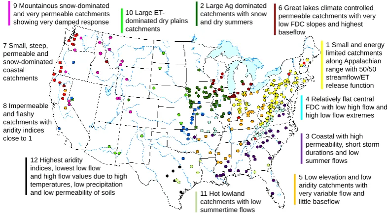
Fig. 1. Results of cluster analysis based on 6 hydrological signatures.
assignment generated from the AutoClass clustering result (Banjeree et al., 2008). The stopping criteria used to prune the tree was 10-fold cross validation. Limitations to the CART analysis, resulting from simplistic splits and a small number of catchments in two of the classes (C11 and C12), were adjusted manually to improve accuracy and value of the analysis.
4 Results and discussion
4.1 Catchment classification for baseline decade (1948–1958)
The AutoClass cluster analysis produced 12 classes as shown in Fig. 1. The normalized influence measure discussed in the Methods section quantifies the importance of a signature for the clustering result. The signatures influenced the cluster analysis in descending order [Signature (Normalized Influ-ence Measure)]:RQP(1.00),RSD(0.807),SFDC(0.626),BFI
(0.626),Q90 (0.626), andQ10 (0.501). The spatial patterns
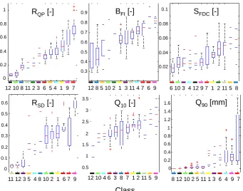
found are generally similar to the ones identified in Sawicz et al. (2011), though some differences are present due to the changes in signatures and catchments, i.e., we use a larger and more diverse set of catchments in this study. First we briefly discuss the classification for the baseline period in detail, and subsequently focus on class changes for the other decades. Qualitative statements regarding whether signature values and physical/climatic characteristics are high or low are only made in relation to other catchments within our data set (Fig. 2 and Supplement).
The classes exhibit strong spatial patterns in most cases (Fig. 1). A collection of small catchments in the northeast and along the north-facing side of the Appalachians form a sin-gle cluster, which are characterized by their energy-limited hydrology (class C1). In contrast to C1, class C2 consists of large agricultural catchments that experience both signifi-cant snow storage during the winter and have very dry sum-mers. The next cluster of catchments, with a relatively wide spatial spread, is found along the southeast coast of the US and is characterized by the permeable geology of this region, which is reflected in their flat flow duration curves (FDC) and relatively high baseflow (class C3) (Bloomfield et al., 2009). These catchments experience short duration precipi-tation events and dry summers that result in significant low flow periods. Directly south of class C3, we identify a cluster of catchments on the south-facing slopes of the Appalachi-ans with low high flows (Q10) and high low flows (Q90;
class C4), and hence flat FDCs similar to C3, but with dif-ferent precipitation characteristics. Catchments of class C5 are located further inland and at lower elevations from C4, thus having low aridity, highly variable streamflow and little baseflow due to fairly impermeable soils. Class C6 is a clus-ter of catchments located on the southern side of the Great Lakes. The Great Lakes play a major role in the climate of the region and the catchments experience very low values of
SFDC as well as the highest values of BFI. Catchments
0.1
0.08
0.06
0.04
0.02
12 10 8 11 2 3 6 5 4 1 9 7 12 8 5 10 2 1 3 11 4 7 6 9 6 10 3 4 12 9 7 1 2 11 5 8
11 12 3 5 4 8 10 2 1 6 7 9 12 10 4 6 3 8 7 1 2 11 5 9 8 12 10 2 5 11 1 3 6 4 9 7
Class
R
QP[-]
B
FI[-]
S
FDC[-]
R
SD[-]
Q
10[-]
Q
90[mm]
1
0.8
0.6
0.4
0.2
0
0.3 0.4 0.5 0.6 0.7 0.8 0.9
0.4
0.3
0.2
0.1
0 0.5 0.6
2.5
2
1.5
1
0.5 3 3.5
[image:5.595.128.470.60.328.2]0 0.2 0.4 0.6 0.8 1 1.2 1.4 1.6
Fig. 2. Box–whisker plots of signature characteristics for the different clusters.
C7 are also snow dominated and exhibit the highest runoff ra-tios. Class C8 shows an interesting separation between a few catchments located in the western US and a bigger cluster lo-cated in the central US. Catchments in C8 are characterized by impermeable soils, which cause a flashy response, while their aridity indices are close to 1. Class C9 consists of mountainous catchments with the highest elevations in the northern US. These are heavily snow-dominated catchments (highest ratio of snow days) with a very damped (highest per-centage sand in soils) and delayed response to precipitation input. The largest catchments by area are part of class C10. Catchments in C10 are located in the central and southwest-ern US and have an ET-dominated climate (lowest precip-itation) (ET: evapotranspiration). Class C11 is made up of catchments found at the lowest elevations within the data set, which experience the highest temperatures and exhibit very low summertime flows. The final cluster of catchments (class C12) experiences the highest aridity indices (lowest runoff ratio), the lowest high flows (Q10) and lowest
base-flow indices. This hydrologic behavior is caused by high air temperature, low precipitation amounts and low permeability soils.
4.2 CART analysis to understand class separations
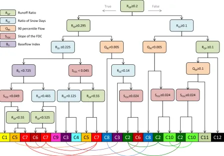
Figure 3 shows the decision tree resulting from a CART anal-ysis of the clustering for the baseline decade discussed above. A total of 285 catchments (91 %) could be correctly assigned
via the decision tree for the original AutoClass classifica-tion (Fig. 4), which resulted in 21 different end nodes (some classes have more than one end node). The presence of more end nodes than classes is an artifact of the CART analysis itself and the method in which it organizes information.
The thresholds within the decision tree mark key transi-tions between different classes. The runoff ratio threshold of 0.295 represents a primary separation between wet and dry catchments within the classification. The Pike–Turc equation that can be used to estimateRQPfrom estimates ofP/PE is
defined as follows:
RQP =1−
1
1+ P PE
2
1 2
. (1)
Interestingly, when applying this Turc–Pike relationship, a
RQP value of 0.295 represents an expected aridity index
(P/PE) of 1 (Pike, 1964; Gerrits et al., 2009). This threshold can therefore be interpreted as the separation between wa-ter limited (RQP<0.295) and energy limited (RQP>0.295)
catchments. This threshold value was achieved purely as a result of the empirical Autoclass cluster and CART analyses. For the slope of the FDC (SFDC) the primary
separa-tions, at 0.045 and 0.049, are virtually the same on both branches of the classification system.SFDC values less than
this threshold value correspond to a more “filtered or damped response” whereas larger values correspond to a more “flashy response”.SFDCrepresents the distribution of flow values of
True False
C1 C5 C7 C6 C7 C9
BFI <0.725
SFDC <0.049
RQP<0.55
RSD<0.465
RSD ≥0.225
RQP<0.525
SFDC < 0.045
RSD<0.125 RQP<0.55
Q90<0.005
RSD<0.14
SFDC≥0.024
RQP ≥0.1
RSD≥0.1
Q90≥0.1
C3 C4
RQP≥0.2
RQP≥0.295
C5 C7 C8 C3 C2 C6 C11 C12
Q90<0.005
SFDC≥0.024
C10 C2 C8
RSD
RQP
Q90
SFDC
BFI
Runoff Ratio
Ratio of Snow Days
90 percentile Flow
Slope of the FDC
Baseflow Index
SFDC≥0.024
[image:6.595.73.523.65.378.2]C10 C2
Fig. 3. The CART decision tree shows the classification tree based on the values of signatures used in this study. This structure is utilized to model the results of the AutoClass clustering algorithm for predicative capability.
C0 C1 C2 C3 C4 C5 C6 C7 C8 C9 C10 C11 0
20 40 60 80 100
Decision Tree Class Assignment
C
la
s
s
A
s
s
ig
n
m
e
n
t
[%
]
Number of Catchments in each Bin
76 45 35 35 29 21 10 22 22 7 7 5
C1 C2 C3 C4 C5 C6 C7 C8 C9 C10 C11 C12 Decision Tree Class Assignment
Fig. 4. Analysis of CART analysis results with respect to the per-centage of classes that have been assigned (correct assignment: min is 76 %; avg. is 91 %). Colors are used to show misclassification through CART.
in the distribution of precipitation events or by land use change that can alter how a catchment partitions water at the land surface.
The ratio of snow days,RSD, with a threshold of 0.225,
can be interpreted as the length of winter conditions. With the exception of the catchments in the western US, which ex-perience a dramatically different distribution of precipitation (dominant winter precipitation), there is a clear relationship betweenRSD and the length of time between the first day
of freezing and first day of thawing. ARSDvalue of 0.225
equals approximately 4 months of snow conditions (less than 0.225 can be considered to be a short winter, and greater than 0.225 can be considered a long winter). Unlike the other signature thresholds, there is more than one RSD threshold
present in the regression tree. A threshold of 0.125 corre-sponds to a duration of about 3 months, while a threshold of 0.465 corresponds to 5–6 months of winter conditions.
The low flow characteristic Q90 only appears in the
re-gression tree to separate catchments that have zero flow peri-ods from those that show perennial streamflow, at a threshold of 0.005. This corresponds to a separation between perennial or near perennial catchments (Q90>0.005) and intermittent
streams (Q90<0.005), i.e., those that experience streamflow
less than 90 % of the time (Laaha and Bloschl, 2006). The second flow percentile,Q10, does not appear in the CART
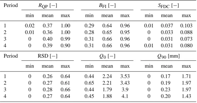
[image:6.595.49.285.430.582.2]Table 2. Minimum, mean, and maximum values for the six signature classes across each of the four periods.
Period RQP[−] BFI[−] SFDC[−]
min mean max min mean max min mean max
1 0.02 0.37 1.00 0.29 0.64 0.96 0.01 0.037 0.103 2 0.01 0.36 1.00 0.28 0.65 0.95 0 0.033 0.088 3 0 0.40 0.99 0.31 0.66 0.96 0 0.031 0.073 4 0 0.39 0.90 0.31 0.66 0.96 0.01 0.031 0.080
Period RSD[−] Q0[−] Q90[mm]
min mean max min mean max min mean max
1 0 0.26 0.64 0.44 2.24 3.53 0 0.17 1.71 2 0 0.27 0.61 0.65 2.21 3.43 0 0.19 1.97 3 0 0.28 0.66 0.44 1.79 3.9 0 0.23 1.97 4 0 0.27 0.64 0.45 1.88 4.1 0 0.20 1.43
4.3 Signature values during the four decades
A wide range of climatic and physical catchment character-istics impacts hydrologic signature values (Wagener et al., 2007). Disentangling these influences simultaneously for a large number of catchments is likely to be very difficult given the lack of time series describing land use patterns such as urbanization (e.g., Martin et al., 2012) and due to the heterogeneity of characteristics found within a catch-ment (especially those that are poorly described, such as subsurface characteristics). Nonetheless we characterize the changes observed, and make an attempt here to explain some of the identified changes. We focus on how some of these shortcomings of empirical studies can be overcome by phys-ically based modeling in a parallel study (Troch et al., 2013). The potential impact of both climate and land use change on hydrologic signatures is briefly discussed before we iden-tify the signature value (and class) changes in our data set. Many studies have generally reported an increase in stream-flow in the US during the latter half of the 20th century in both gradual and sudden (step) changes (McCabe and Wolock, 2002). Between 1948 and 1988, regions across the US experienced varied changes in land use, including ur-banization, deforestation and vegetation clearance (south-ern US), forest and vegetation regrowth (south(south-ern and east-ern US), and expanding agricultural cover (midwesteast-ern US) (Woodbury et al., 2006; Allan, 2004; Garbrecht et al., 2004; Drummond and Loveland, 2010; Mitchell and Dun-can, 2009). These changes have altered catchment behavior by impacting the primary hydrologic functions of partition-ing, storage and release of water. As an example, deforesta-tion can increase soil water storage while simultaneously de-creasing the amount of water leaving a catchment through the extraction of soil moisture from vegetative transpiration (Fohrer et al., 2001). In the midwest, agriculture has tran-sitioned from mixed perennial and annual cropping systems to primarily annual crops (Schilling et al., 2008). Increasing
agricultural activity has been found to increase evapotranspi-ration and to change soil water retention and the length and distribution of flow paths (Garbrecht et al., 2004; Schilling et al., 2008).
Changes to both average and extreme climate conditions will also alter catchment behavior. Streamflow has gener-ally increased across the contiguous US in large part due to changes in average climatic conditions (Lins and Slack, 1999; McCabe and Wolock, 1997; Sun et al., 2008). The flow duration curve is partly influenced by the frequency, inten-sity, or distribution of precipitation events, as these charac-teristics impact the overall distribution of streamflow events (Wang and Wu, 2013; Coopersmith et al., 2012; Ye et al., 2012). Yaeger et al. (2012) found lower flow duration curve slope values when the precipitation regime of a catchment becomes more evenly distributed intra-annually. Generally, warmer winter air temperatures will reduce snow storage, re-sulting in an earlier and less severe spring-melt contribution to streamflow response and removing the presence of large spring-melt events in the streamflow time series. This is more likely to be observed in western catchments because the ma-jority of precipitation for these catchments falls during the winter months (Groisman et al., 2001; Stewart et al., 2005; Hidalgo et al., 2009).
Examination of how the six signatures vary across the four decades (Table 2) informs us of general trends. As an aver-age across all catchments,RQPshows little variation across
the four decades, though some catchments experience large changes between periods (±15 % of the total range). If we examine the degree of change between decades, we find that delta values (change of signature values between decades) are more or less normally distributed between each period, with mean values slightly below zero from the first to sec-ond and third to fourth periods, and slightly positive be-tween the second and third periods.RSDis similarly
delta values between periods 1 and 2 (the remaining differ-ences show normal distributions).BFI changes are normal
distributed with consistently positive means between each of the four decades (with a maximum mean of 1.3 % found between periods 2 and 3). Change values forBFIare greater
than forRQPandRSDwith maximum interperiod variability
reaching 25–30 % of the range over time.SFDCchange
val-ues exhibit a slightly negative skew between each period and show consistently negative means (most extreme mean value of−4 % between periods 1 and 2). The largest value ofSFDC
change reaches−47 % of the total range. The distribution of changes forQ90is positively skewed. However, catchments
that have the highest values also show the greatest variabil-ity (∼30 %).Q10, which is not present in the decision tree,
shows the highest variability through time, with mean values of−1,−11, and 2 % between periods 1 and 2, 2 and 3, and 3 and 4, respectively.Q90 andQ10 are expected to exhibit
the most interperiod variability because they refer to the tails of the distributions whereas the other four signatures either capture flow conditions that are more common (e.g.,SFDC
fo-cuses on central low flows), or capture longer time averages (BFI,RQP,RSD).RQP,BFI, andSFDCall show the least
vari-ability during the final transition phase, whereasRSD,Q90,
andQ10 show the least variability between period 1 and 2. RQP,BFI,RSD,Q10, andQ90exhibit the highest variability
between periods 2 and 3, while we found the highest vari-ability forSFDCbetween periods 1 and 2. The considerable
difference between the mean of the changes and the changes occurring in individual catchments suggests that it is sensible to break the analysis up by geographic region.
4.4 Interpretation of change by region
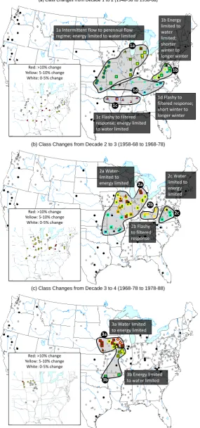
Change in catchment class assignment is organized as three transition phases between each of the four decades studied. We identify groups of catchments that change class assign-ment between decades, rather than focusing on individual catchments in isolation, to better understand broader patterns of change. Trying to explain the change occurring in each in-dividual catchment would be infeasible. During the first tran-sition phase (between period 1 and 2), four spatially inter-esting class changes occur. The second and third transition phases both exhibit two spatially interesting class changes. The groups of catchments that we emphasized, along with the remaining changing catchments are shown in Fig. 5a–c. The inner color of each marker on the maps describes the ini-tial class (see Fig. 1 for color scheme legend) and the border color describes the new class in which catchments transition during the decade under study.
4.4.1 Transition phase 1 (1948–1958 to 1958–1968)
The first group of catchments we analyze is located in the midwest/Great Lakes area. Its members transition from a number of different classes (C1, C4, C5, C6, C8) to a single
class, (C2, indicated by the dark green marker border; Figs. 5 and 1a). These changes in hydrologic similarity can be ex-plained by changes to runoff ratio,RQP (C1, C4, and C5),
and to low flows,Q90 (C8). For the latter, a small increase
in average precipitation (5 %) changes C8 (shown as blue in-side of the marker) catchments to C2 catchments due to a slight increase in Q90. The intra-annual variability of
pre-cipitation on average does not change during this transition period, so it is a general increase of precipitation that seems to explain the increase inQ90. These catchments are located
across Missouri, Oklahoma, and Kansas and exhibit high per-centages of agricultural land use (57.5 % for Kansas, 42.5 % in Missouri, and 34 % in Oklahoma) (Nickerson et al., 2011). However, the change inQ90does not seem to be affected by
the change of land use as changes to agricultural cover be-tween these two periods of time are inconsistent across these three states, with Missouri agricultural land showing an in-crease, Oklahoma cover a dein-crease, and the Kansas cover re-maining constant (Nickerson et al., 2011). The primary rea-sons for this shift appear to be the increase in precipitation in general (from period 1 to period 2) and an increase in sum-mer rainfall specifically (Pryor and Schoof, 2008).
Shifts in catchments from one class to many or from many classes to one between phases often seem to be tied to shifts between water and energy limited conditions. Initially, the catchments during the first transition separate into classes C1, C4, C5, and C6 due to the difference in values ofSFDC, BFI, andRSD. The energy-limited catchments are further
sep-arated from the water-limited catchments belonging to C2 (dark green marker border) during the baseline period. How-ever, the dissimilarity inSFDC,BFI, andRSDvalues became
secondary to the common shift of the aridity index to a water-limited state, and the corresponding change in runoff ratio,
RQP, resulting in catchments from many classes shifting to a
single class. The primary cause of this decrease inRQP
val-ues was a decrease in total annual precipitation (mean annual decrease of about 8 %).
Catchments located in Virginia diverge from class C4 (cyan) into classes C2 and C1 (Figs. 5, 1b). The shift from C4 to C2, caused by a decrease inRQPvalues, is most likely
driven by an average 9 % decrease in precipitation across these catchments. In contrast, catchments that transition from C4 to C1 do so due to higher values of ratio of snow days (RSD) (increasing past the 0.225 threshold), which
corre-sponds to a two week increase in winter length. The increase inRSDvalues is caused by a decrease in air temperature by
an average of 0.7◦C. All catchments transitioning from class
C4 to C2 and C1 experience the same mean increase in their
RSDvalues (average of 0.03). However, the initialRSDvalues
vary from 0.14 to 0.22. This increase results in a divergence of classes as theRSD values for the second period (range
1a Intermittent flow to perennial flow regime; energy limited to water limited
1b Energy limited to water limited; shorter winter to longer winter
1d Flashy to filtered response; short winter to longer winter 1c Flashy to filtered
response; energy limited to water limited
1a
1b
1d
1c
(a) Class Changes from Decade 1 to 2 (1948-58 to 1958-68)
Red: >10% change Yellow: 5-10% change
White: 0-5% change
2a Water-limited to energy limited
2b Flashy to filtered response
2c Water limited to energy limited
2a
2b
2c
(b) Class Changes from Decade 2 to 3 (1958-68 to 1968-78)
Red: >10% change Yellow: 5-10% change
White: 0-5% change
3a Water limited to energy limited
3b Energy limited to water limited
3a
3b
(c) Class Changes from Decade 3 to 4 (1968-78 to 1978-88)
Red: >10% change Yellow: 5-10% change
[image:9.595.156.442.67.677.2]White: 0-5% change
elevations) whereas the catchments transitioning to C2 are found directly east of the mountain range (lower elevations). Southeastern US catchments, originally part of class C5 (orange), transition to C3 mainly due to a change inSFDC
(four catchments) (Figs. 5, 1c). The behavioral distinction between these classes isSFDC, which shows a more damped
response in these catchments during the second period, as opposed to a more flashy response in the baseline period (three of the four catchments experience a decrease of over 10 % of the observed range). These catchments also expe-rience a mean precipitation seasonality index (PSI [−]), a measure of seasonality of precipitation) across all catchments of 0.21 during the first period and 0.19 during the second period (Pryor and Schoof, 2008). This represents a 2.4 % de-crease in the seasonality of precipitation throughout the year, which may contribute, as a minor part, to the more damped response observed.
The last observed shift during the first transition phase oc-curs through parts of Arkansas, Mississippi, and Alabama, where catchments in classes C3 and C5 transition to class C4 (Figs. 5, 1d). Catchments transitioning from C5 show a decrease inSFDC(which again indicates a more damped
re-sponse as was seen in area 1c). These catchments experience a decrease in PSI, from an average of 0.19 in the first pe-riod to 0.165 to the next pepe-riod. However, even though the mean values of these catchments are decreasing, two of the four catchments do not experience any change in PSI imply-ing that there must be other causes for the decrease inSFDC,
which we cannot identify from our database. They do not transition to C3, as they experience a higher value ofRSD
than those in 1c. Catchments, which transition from C3 to C4, experience an increase inRSDdue to a two-week
aver-age lengthening of the winter season per year.
4.4.2 Transition phase 2 (1958–1968 to 1968–1978)
A reversal of some of the observed changes from transition period 1 occurs. Catchments belonging to C2 (dark green) in the second period experience transitions to a number of classes (C1, C4, C5, and C6; Fig. 5b, groups 2a and 2c), shift-ing back from water to energy-limited conditions due to an increase inRQP. The cause of this shift can be attributed to an
average increase of annual precipitation of 0.24 mm day−1. This transition is seen both in areas 2a and 2c, which cover the midwest/Great Lakes region and the eastern slopes of the Appalachian Mountains.
Catchments located in West Virginia and Kentucky be-longing to class C5 (orange) show a shift from a flashy re-sponse in the second period to a more damped rere-sponse in the third period, quantified by a decrease in theSFDCvalues
for these catchments (Figs. 5b, 2b). Catchments transition to C1 (yellow) and C4 (cyan), depending on whether the value ofRSDfor each of these catchments is above (C4) or below
(C1) the 0.225 regression tree threshold. These catchments experience a relatively large decrease in PSI (0.20 in period 2
vs. 0.14 in period 3), which suggests that the cause of the de-crease inSFDCis a less seasonal precipitation regime.
4.4.3 Transition phase 3 (1968–1978 to 1978–1988)
Changes occurring between the third and fourth periods are again dominated by shifts between water and energy limited conditions across the midwest. Despite close spatial proxim-ity, the northern portions of Iowa experience a slight increase in precipitation (2 % from the prior period), while the south-ern portion of Iowa, the eastsouth-ern portion of Illinois, and all catchments in Missouri and Arkansas experience a decrease (3 % from the prior period) in precipitation. These changes result in proportional shifts inRQPvalues and hence in class
transitions. Catchments located in central to northern Iowa (Figs. 5, 3a) transition from C1 (yellow) to C6 (dark red), while the remaining catchments of interest transition from C4 (cyan) to C2 (dark green). Changes inRQP values that
cause these transitions are much smaller than those found in other phases though (±1 to 2 %). These transitions therefore highlight how even small changes in climate can result in different shifts in behavior for neighboring catchments. Al-though land use in this general area is dominated by agricul-ture, there is no substantial change in agricultural land use at the state level during the third transition period (Nickerson et al., 2011), and no general trends were found that suggested agriculture had an effect onRQP.
Strong spatial patterns were found for groups of catch-ments that transition between classes for similar reasons, al-beit the magnitudes of those changes differ in relation to the catchments’ proximity to thresholds in the signature space. As described above, changes to climatic forcing are primar-ily responsible for spatial patterns of shifts in catchment be-havior. However, there are a number of catchments that did not experience behavioral shifts found in other similar catch-ments. These catchments have experienced changes in sig-nature values for reasons that we were unable to quantify at present. Catchments along the western coast experience a high climatic gradient as well as variable local physical features. In order to interpret the control of class transition in these catchments over time, we require additional tempo-ral information quantifying changes in how vegetation, land use, and human activity change.
5 Conclusions and open questions
and daily timescales to classify catchment behavior across the US. We find that catchments experienced changes to all six signatures to differing degrees at different times.
The initial classification for the baseline decade (1948– 1958) resulted in 12 clusters that are distinctly separated due to differences in hydrological behavior as expressed by the signature values. We subsequently analyzed how much other decades deviate from this initial classification by re-classifying the catchments using a decision-tree established for the baseline period. The first transition phase, taking place between 1948–1958 and 1958–1968, showed just over 40 of the 314 catchments changing class, geographically ranging from Oklahoma/Nebraska to Virginia. The second transition phase, between 1958–1968 and 1968–1978, has a similar number of class changing catchments, mostly experi-encing large changes (5–10 %) in values ofRQPandSFDC.
During the last transition phase, between 1968–1978 and 1978–1988, only about half as many catchments changed class, and they were located solely in the midwest.
Generally, climate was found to be a primary control on catchment behavior when comparing catchments at the decadal scale. Change in climatic characteristics – mean annual precipitation, length of winter period, intra-annual seasonality of precipitation – had the strongest impact on changes in catchment behavior. While we were able to ex-plain some of the changes found, e.g., the regular switch be-tween energy- and water-controlled regimes for catchments close to an aridity index of one, other temporal variability could not be explained as well with the information avail-able. For example, changes to the flow duration curve slope,
SFDC, could be caused by a multitude of different factors and
we could not shed light on which one dominates. Land use, although likely to be important in how a catchment filters water, was not found to provide valuable information in de-scribing the change in hydrologic behavior (most likely due to limited information available at the catchment scale). The difficulty in explaining some of the changes based on an empirical analysis alone, as attempted here, might also par-tially relate the rather moderate changes observed. Martin et al. (2012), for example, showed that urbanization in the or-der of 15 % of the total catchment area could be required to produce a significant change in signature characteristics. This might explain why we mainly find climatic character-istics to matter, which, by definition, occur across the whole catchment rather than a small part of it as often the case for land use change. It leads us again to the conclusion, simi-larly as in Sawicz et al. (2011), that an empirical analysis of the type shown here is a nice first step to understanding con-trols (and therefore change). However, it is likely that a sub-sequent analysis using a mechanistic model is required given the limits of data available for describing the heterogeneity of catchment characteristics in space and time.
Supplementary material related to this article is
available online at http://www.hydrol-earth-syst-sci.net/ 18/273/2014/hess-18-273-2014-supplement.pdf.
Acknowledgements. The National Science Foundation under project EAR-0635998, Understanding the Hydrologic Implications of Landscape Structure and Climate – Towards a Unifying Frame-work of Watershed Similarity, provided support for this project. Time series data used in this study was provided by the MOPEX project.
Edited by: E. Zehe
References
Allan, D. J.: Landscapes and riverscapes: the influence of land use on stream ecosystems, Ann. Rev. Evol. Syst., 35, 257–284, doi:10.1146/annurev.ecolsys.35.120202.110122, 2004.
Andreassian, V.: Waters and Forests: From Historical Controversy to Scientific Debate, J. Hydrol., 291, 1–27, 2004.
Archcar, F., Camadro, J., and Mertivier, D.: AutoClass@IJM: a powerful tool for Bayesian classification of heterogeneous data in biology, Nucl. Acids Res., 37, 1–5, doi:10.1093/nar/gkp430, 2009.
Banerjee, A. K., Arora, N., and Murty, U. S. N.: Classification and regression tree (CART) analysis for deriving variable importance of parameters influencing average flexibility of CaMK kinase family, Electron. J. Biol., 4, 27–33, 2008.
Bloomfield, J. P., Allen, D. J., and Griffiths, K. J.: Examining geo-logical controls on baseflow index (BFI) using regression analy-sis: an illustration from the Thames Basin, UK, J. Hydrol., 353, 164–176, doi:10.1016/j.jhydrol.2009.04.025, 2009.
Carrillo, G., Troch, P. A., Sivapalan, M., Wagener, T., Harman, C., and Sawicz, K.: Catchment classification: hydrological analysis of catchment behavior through process-based modeling along a climate gradient, Hydrol. Earth Syst. Sci., 15, 3411–3430, doi:10.5194/hess-15-3411-2011, 2011.
Cheeseman, P. and Stutz, J.: Bayesian Classification (AutoClass): Theory and Results, in: Advances in Knowledge Discovery and Data Mining, edited by: Fayyad, U. M., Piatetsky-Shapiro, G., Smyth, P., and Uthurusamy, R., AAAI Press/MIT Press, Cam-bridge, 1996.
Cheng, L., Yaeger, M., Viglione, A., Coopersmith, E., Ye, S., and Sivapalan, M.: Exploring the physical controls of re-gional patterns of flow duration curves – Part 1: Insights from statistical analyses, Hydrol. Earth Syst. Sci., 16, 4435–4446, doi:10.5194/hess-16-4435-2012, 2012.
Coopersmith, E., Yaeger, M. A., Ye, S., Cheng, L., and Sivapalan, M.: Exploring the physical controls of regional patterns of flow duration curves – Part 3: A catchment classification system based on regime curve indicators, Hydrol. Earth Syst. Sci., 16, 4467– 4482, doi:10.5194/hess-16-4467-2012, 2012.
Corduas, M.: Clustering streamflow time series for regional classification, J. Hydrol., 407, 73–80, doi:10.1016/j.jhydrol.2011.07.008, 2011.
Duan, Q., Schaake, J., Andreassian, V., Franks, S., Goteti, G., Gupta., H. V., Gusev, Y. M., Habets, F., Hall, A., Hay, L., Hogue, T., Huang, M., Leavesley, G., Liang, X., Nasonova, O. N., Noi-han, J., Oudin, L., Soroochian, S., Wagener, T., and Wood, E. F.: Model Parameter Estimation Experiment (MOPEX): An overview of science strategy and major results from the second and third workshops, J. Hydrol., 320, 1–15, 2005.
Falcone, J. A., Carlisle, D. M., Wolock, D. M., and Meador, M. R.: Gages: A stream gage database for evaluating natural and altered flow conditions in the conterminous United States, Ecology, 91, 2010.
Flury, M. and Wai, N. N.: Dyes as tracers for vadose zone hy-drology, Rev. Geophys., 41, 1002, doi:10.1029/2001RG000109, 2003.
Fohrer, N., Haverkamp, S., Eckhardt, K., and Frede, H. G.: Hydro-logic response to land use changes on the catchment scale, Phys. Chem. Earth B, 26, 577–582, 2001.
Garbrecht, J. D., Van Liew, M., and Brown, G. O.: Trends in precip-itation, streamflow, and evapotranspiration in the Great Plains of the United States. J. Hydrol. Eng., 9, 360–367, 2004.
Gerrits, A. M. J., Savenije, H. H. G., Veling, E. J. M., and Pfister, L.: Analytical derivation of the Budyko curve based on rainfall characteristics and a simple evaporation model, Water Resour. Res., 45, W04403, doi:10.1029/2008WR007308, 2009. Gharari, S., Hrachowitz, M., Fenicia, F., and Savenije, H. H. G.:
Hydrological landscape classification: investigating the perfor-mance of HAND based landscape classifications in a central European meso-scale catchment, Hydrol. Earth Syst. Sci., 15, 3275–3291, doi:10.5194/hess-15-3275-2011, 2011.
Groisman, P. Y., Knight, R. W., and Karl, T. R.: Heavy precipitation and high streamflow in the contiguous United States: trends in the twentieth century, B. Am. Meteorol. Soc., 82, 219–246, 2001. Haines, A. T., Finlayson, B. L., and McMahon, T. A.: A global
clas-sification of river regimes, Appl. Geogr., 8, 255–272, 1988. He, Y., Bárdossy, A., and Zehe, E.: A review of regionalisation for
continuous streamflow simulation, Hydrol. Earth Syst. Sci., 15, 3539–3553, doi:10.5194/hess-15-3539-2011, 2011.
Hidalgo, H. G., Das, T., Dettinger, M. D., Cayan, D. R., Pierce, D. W., Barnett, T. P., Bala, G., Mirin, A., Wood, A. W., Bon-fils, C., Santer, B. D., and Nozawa, T.: Detection and At-tribution of Streamflow Timing Changes to Climate Change in the Western United States, J. Climate, 22, 3838–3855, doi:10.1175/2009JCLI2470.1.2009, 2009.
Hubert, L. and Arabie, P.: Comparing partitions, J. Classificat., 2, 193–218, 1985.
Kennard, M. J., Mackay, S. J., Pusey, B. J., Olden, J. D., and Marsh, N.: Quantifying uncertainty in estimation of hydrologic metrics, River Res. Appl., 26, 137–156, 2010.
Laaha, G. and Bloschl, G.: A comparison of low flow regional-ization methods-catchment grouping, J. Hydrol., 323, 193–214, doi:10.1016/j.jhydrol.2005.09.001, 2006.
Ley, R., Casper, M. C., Hellebrand, H., and Merz, R.: Catch-ment classification by runoff behaviour with self-organizing maps (SOM), Hydrol. Earth Syst. Sci., 15, 2947–2962, doi:10.5194/hess-15-2947-2011, 2011.
Lins, H., and Slack, J. R.: Streamflow trends in the United States, Geophys. Res. Lett., 26, 227–230, 1999.
Mahmood, R., Foster, S. A., Keeling, T., Hubbard, K. G., Carlson, C., and Leeper, R.: Impacts of irrigation on 20thcentury tem-perature in the northern Great Plains, Global Planet. Change, 54, 1–18, 2006.
Martin, E. H., Kelleher, C., and Wagener, T.:Has Ur-banization changed ecological streamflow characteris-tics in Maine (USA)?, Hydrolog. Sci. J., 57, 1–18, doi:10.1080/02626667.2012.707318, 2012.
McCabe, G. J. and Wolock, D. M.: Climate change and the detection of trends in runoff, Clim. Res., 8, 129–134, 1997.
McCabe, G. J. and Wolock, D. M.: A step increase in the con-terminous United States, Geophys. Res. Lett., 29, 38-1–38-4, doi:10.1029/2002GL015999, 2002.
McDonnell, J. J. and Woods, R.: On the need for catchment classifi-cation, J. Hydrol., 299, 2–3, doi:10.1016/j.jhydrol.2004.09.003, 2004.
Merz, R., Parajka, J., and Blöschl, G.: Time stability of catchment model parameters: Implications for climate impact analyses, Water Resour. Res., 47, W02531, doi:10.1029/2010WR009505, 2011.
Milly, P. C. D., Betancourt, J., Falkenmark, M., Hirsch, R. M., Kundzewicz, Z. W., Lettenmaier, D. P., and Stouffer, R. J.: Sta-tionarity is dead: Whither water management?, Science, 319, 573–574, 2008.
Mitchell, R. J. and Duncan, S. L.: Range of variability in southern coastal plain forests: its historical, contemporary, and future role in sustaining biodiversity, Ecol. Soc., 14, 17, 2009.
Moliere, D. R., Lowry, J. B. C., and Humphrey, C. L.: Classifying the flow regime of data-limited streams in the wet-dry tropical region of Austraila, J. Hydrol., 367, 1–13, 2009.
Nickerson, C., Ebel, R., Borchers, A., and Carriazo, F.: Major Uses of Land in the United States, 2007, EIB-89, US Department of Agriculture, Economic Research Service, 2011.
Olden, J. D., Kennard, M. J., and Pusey, B. J.: A framework for hydrologic classification with a review of methodologies and ap-plications in ecohydrology, Ecohydrologz, 5, 503–518, 2011. Parton, W. J., Gutmann, M. P., Williams, S. A., Easter, M., and
Ojima, D.: Ecological impact of historical land-use patterns in the Great Plains: A methodological assessment, Ecol. Appl., 13, 1915–1928, 2005.
Pegg, M. A. and Pierce, C. L.: Classification of reaches in the Mis-souri and Lower Yellowstone Rivers based on flow characteris-tics, River Res. Appl., 18, 31–42, 2002.
Pike, J. G.: The estimation of annual runoff from meteorological data in a tropical climate, J. Hydrol., 2, 116–123, 1964. Pryor, S. C. and Schoof, J. T.: Changes in the seasonality of
precipi-tation over the contiguous USA, J. Geophys. Res., 113, D21108, doi:10.1029/2008JD010251, 2008.
Rand, W. M.: Objective criteria for the evaluation of clustering methods, J. Am. Stat. Assoc., 66, 846–850, 1971.
Rosero, E., Yang, Z.-L., Wagener, T., Gulden, L. E., Yatheendradas, S., and Niu, G.-Y.: Quantifying parameter sensitivity, interaction and transferability in hydrologically enhanced versions of Noah-LSM over transition zones, J. Geophys. Res., 115, D03106, doi:10.1029/2009JD012035, 2010.
Sawicz, K., Wagener, T., Sivapalan, M., Troch, P. A., and Carrillo, G.: Catchment classification: empirical analysis of hydrologic similarity based on catchment function in the eastern USA, Hy-drol. Earth Syst. Sci., 15, 2895–2911, doi:10.5194/hess-15-2895-2011, 2011.
Schilling, K. E., Jha, M. K., Zhang, Y.-K., Gassman, P. W., and Wolter, C. F.: Impact of land use and land cover change on the water balance of a large agricultural watershed: Historical ef-fects and future directions, Water Resour. Res., 44, W00A09, doi:10.1029/2007WR006644, 2008.
Ssegane, H., Tollner, E. W., Mohamoud, Y. M., Rasmussen, T. C., and Dowd, J. F.: Advances in variable selection methods I: Causal selection methods versus stepwise regression and princi-pal component analysis on data known and unknown functional relationships, J. Hydrol., 438–439, 16–25, 2012.
Ssegane, H., Tollner, E. W., Mohamoud, Y. M., Rasmussen, T. C., and Dowd, J. F.: Advances in variable selection methods II: Ef-fect of variable selection method on classification of hydrologi-cally similar watersheds in three Mid-Atlantic ecoregions, J. Hy-drol., 438–439, 26–38, 2012.
Stewart, I. T., Cayan, D. R., and Dettinger, M. D.: Changes toward earlier streamflow timing across western North America, J. Cli-mate, 18, 1136–1155, 2005.
Stutz, J. and Cheeseman, P.: AutoClass – a Bayesian Approach to Classification, Maximum Entropy and Bayesian Methods, Cam-bridge 1994, edited by: Skilling, J. and Sibisi, S., Kluwer Ace-demic Publishers, Dordrecht, 1995.
Sun, G., McNulty, S. G., Moore Myres, J. A., and Cohen, E. C.: Impacts of climate, change, population growth, land use, and groundwater availability on water supply and demand across the conterminous U.S., AWRA Hydrology and Watershed Manage-ment Technical Committee, Raliegh, NC, 2008.
Tetzlaff, D., Seibert, J., McGuire, K. J., Laudon, H., Burns, D. A., Dunn, S. M., and Soulsby, C.: How does land-scape structure influence catchment transit time across dif-ferent geomorphic provinces?, Hydrol. Process., 23, 945–953, doi:10.1002/hyp.7240, 2009.
Troch, P. A., Carrillo, G., Sivapalan, M., Wagener, T., and Saw-icz, K.: Climate-vegetation-soil interactions and long-term hy-drologic partitioning: signatures of catchment co-evolution, Hy-drol. Earth Syst. Sci., 17, 2209–2217, doi:10.5194/hess-17-2209-2013, 2013.
Wagener, T.: Can we model the hydrological impacts of environmental change?, Hydrol. Process., 21, 3233–3236, doi:10.1002/hyp.6873, 2007.
Wagener, T., Sivapalan, M., Troch, P. A., and Woods, R. A.: Catch-ment classification and hydrologic similarity, Geogr. Comp., 1, 901–931, 2007.
Wagener, T., Sivapalan, M., Troch, P. A., McGlynn, B. L., Har-man, C. J., Gupta, H. V., Kumar, P., Rao, P. S. C., Basu, N. B., and Wilson, J. S.: The future of hydrology: An evolving sci-ence for a changing world, Water Resour. Res., 46, W05301, doi:10.1029/2009WR008906, 2010.
Wang, D. and Wu, L.: Similarity of climate control on base flow and perennial stream density in the Budyko framework, Hydrol. Earth Syst. Sci., 17, 315–324, doi:10.5194/hess-17-315-2013, 2013.
Webb, J. A., Bond, N. R., Wealands, S. R., McNally, R., Quinn, G. P., Vesk, P. A., and Grace, M. R.: Bayesian clustering with AutoClass explicitly recognizes uncertainties in landscape clas-sification, Ecography, 30, 526–536, 2007.
Winter, T. C.: The concept of hydrologic landscapes, J. Am. Water. Resour. Ass., 37, 335–349, 2001.
Wolock, D. M., Winter, T. C., and Mahon, G.: Delination and evalu-ation of hydrologic-landscape regions in the United States using geographic information system tools and multivariate statistical analyses, Environ. Manage., 34, S71–S88, 2004.
Woodbury, P. B., Heath, L. S., and Smith, J. E.: Land use change effects on forest carbon cycling throughout the southern United States, J. Environ. Qual., 35, 1348-1363, 2006.
Yaeger, M., Coopersmith, E., Ye, S., Cheng, L., Viglione, A., and Sivapalan, M.: Exploring the physical controls of regional pat-terns of flow duration curves – Part 4: A synthesis of empiri-cal analysis, process modeling and catchment classification, Hy-drol. Earth Syst. Sci., 16, 4483–4498, doi:10.5194/hess-16-4483-2012, 2012.