www.hydrol-earth-syst-sci.net/17/4121/2013/ doi:10.5194/hess-17-4121-2013
© Author(s) 2013. CC Attribution 3.0 License.
Hydrology and
Earth System
Sciences
Statistical analysis and modelling of surface runoff from arable
fields in central Europe
P. Fiener1, K. Auerswald2, F. Winter3, and M. Disse4
1Institut für Geographie, Universität Augsburg, 86135 Augsburg, Germany
2Lehrstuhl für Grünlandlehre, Technische Universität München, Alte Akademie 12,
85350 Freising-Weihenstephan, Germany
3Dorsch International Consultants, Hansastr. 20, 80686 Munich, Germany
4Lehrstuhl für Hydrologie und Flussgebietsmanagement, Technische Universität München,
Arcisstraße 21, 80333 Munich, Germany
Correspondence to: K. Auerswald ([email protected])
Received: 25 February 2013 – Published in Hydrol. Earth Syst. Sci. Discuss.: 19 March 2013 Revised: 29 August 2013 – Accepted: 5 September 2013 – Published: 23 October 2013
Abstract. Surface runoff generation on arable fields is an im-portant driver of flooding, on-site and off-site damages by erosion, and of nutrient and agrochemical transport. In gen-eral, three different processes generate surface runoff (Hor-tonian runoff, saturation excess runoff, and return of subsur-face flow). Despite the developments in our understanding of these processes it remains difficult to predict which processes govern runoff generation during the course of an event or throughout the year, when soil and vegetation on arable land are passing many states. We analysed the results from 317 rainfall simulations on 209 soils from different landscapes with a resolution of 14 286 runoff measurements to deter-mine temporal and spatial differences in variables governing surface runoff, and to derive and test a statistical model of surface runoff generation independent from an a priori se-lection of modelled process types. Measured runoff was re-lated to 20 time-invariant soil properties, three variable soil properties, four rain properties, three land use properties and many derived variables describing interactions and curvi-linear behaviour. In an iterative multiple regression proce-dure, six of these properties/variables best described initial abstraction and the hydrograph. To estimate initial abstrac-tion, the percentages of stone cover above 10 % and of sand content in the bulk soil were needed, while the hydrograph could be predicted best from rain depth exceeding initial ab-straction, rainfall intensity, soil organic carbon content, and time since last tillage. Combining the multiple regressions to estimate initial abstraction and surface runoff allowed
mod-elling of event-specific hydrographs without an a priori as-sumption of the underlying process. The statistical model de-scribed the measured data well and performed equally well during validation. In both cases, the model explained 71 and 58 % of variability in accumulated runoff volume and in-stantaneous runoff rate (RSME: 5.2 mm and 0.23 mm min−1, respectively), while RMSE of runoff volume predicted by the curve number model was 50 % higher (7.7 mm). Stone cover, if it exceeded 10 %, was most important for the ini-tial abstraction, while time since tillage was most impor-tant for the hydrograph. Time since tillage is not taken into account either in typical lumped hydrological models (e.g. SCS curve number approach) or in more mechanistic mod-els using Horton, Green and Ampt, or Philip type approaches to address infiltration although tillage affects many physical and biological soil properties that subsequently and gradu-ally change again. This finding should foster a discussion re-garding our ability to predict surface runoff from arable land, which seemed to be dominated by agricultural operations that introduce man-made seasonality in soil hydraulic properties.
1 Introduction
EUROSTAT, 2012). Runoff generation is the driver of on-site and off-site damages by erosion processes and of nutrient and agrochemical transport (e.g. Haygarth et al., 2006) into open water bodies especially during local floods (e.g. Evrard et al., 2008). Thus, surface runoff generation on arable land is important for hydrological modelling, especially when water quality is considered.
In general, it is acknowledged that three mechanisms gen-erate surface runoff (Li et al., 2012): (i) unsaturated surface runoff (Hortonian-type runoff), (ii) saturation-excess surface runoff, and (iii) return of subsurface storm flow, where the last is detectable in some cases already on the plot scale but becomes increasingly important when moving from the plot to the catchment scale and from the event to longer time scales. Not all excess water generated by these mech-anisms contributes to surface runoff because some is stored on the surface as depression storage (infiltrating after rain events) and detention storage (partly running off after events) (Mohamoud et al., 1990). On the catchment scale, surface runoff partly re-infiltrates along its pathway to the stream network (runon infiltration; e.g. Nahar et al., 2008). Many models are available to address one or more of these mecha-nisms. These include relatively simple approaches that lump all processes operating along the flow path (e.g. the SCS curve number; Mockus, 1972) on a daily time scale or more mechanistic approaches on much shorter time scales (min-utes) addressing a specific process that creates excess water, like models of the Green and Ampt (1911), Philip (1969) or Horton (1940) type. The mechanistic models may then be applied in a spatially distributed context including fur-ther processes occurring during runoff accumulation (for an extensive model overview see, e.g., Borah and Bera (2003); Migliaccio and Srivastava (2007); or the various results from the “distributed model inter-comparison project” (Smith et al., 2004)). Small-watershed-scale models dealing with sur-face runoff and soil erosion from arable land often stick to Hortonian-type surface runoff generation approaches (As-souline and Mualem, 2006; Fiener et al., 2008), assuming that surface sealing during heavy rainfall events dominates runoff generation on partly bare soils. Larger-scale models typically use Green and Ampt or Philip approaches assuming that infiltration is governed by a propagating wetting front depending on soil properties within the soil column (e.g. Kale and Sahoo, 2011; Klar et al., 2008). However, as pro-cesses dominating infiltration and surface runoff generation may vary inter- and intra-annually (Li et al., 2012; Vivoni et al., 2007) and even within an event (e.g. Silburn and Con-nolly, 1995), it is important to address potential switches be-tween runoff generation mechanisms in advanced modelling approaches (Li et al., 2012; Tian et al., 2012).
Despite the improvements of modelling approaches to ad-dress different mechanisms of surface runoff generation si-multaneously (e.g. the THREW model; Li et al., 2012), it remains challenging to account for the specific temporal and spatial variability of soil and crop characteristics in
agricul-tural landscapes (Fiener et al., 2011a; Green et al., 2003), which may affect infiltration. This challenge results from the interaction with agronomic decisions dominating the soil– vegetation system by influencing (i) the seasonal variabil-ity of soil properties and surface roughness depending on tillage operations and (ii) the associated seasonality of plant growth. The first relates to the mostly texture-based, static estimates of important soil variables, e.g. porosity, used in many modelling approaches. The second is associated with the seasonality of plant and residue cover potentially protect-ing the soils from crustprotect-ing (for a review see Fiener et al., 2011a). Despite the developments in our understanding of individual processes in specific cases, it remains difficult to predict which processes govern runoff generation while soil and vegetation are passing many states during a crop rotation. The major objectives of this study were (i) to statistically analyse 317 hydrographs from rainfall simulations carried out on different arable soils covering many landscapes with different crops to determine temporal and spatial differences in variables governing surface runoff during rainfall events and (ii) to derive and test a statistical model of surface runoff generation independent from an a priori selection of mod-elled processes. This model should operate on the plot scale (1–10 m2) for the event scale with a resolution of minutes to obtain hydrographs, but it should take into account the varia-tion of driving variables that happens on the scale of crop ro-tations and the catchment scale. To become operational, e.g. while implementing the plot approach into a distributed event model, it has to rely on variables that usually are available or can be made available on these temporal and spatial scales. This also requires choosing a statistical model and not a pro-cess model, because it would be impossible on these scales to identify the underlying processes. For instance, a return flow had been identified on some plots by the use of trac-ers despite a plot length of only 4.5 m (Haider, 1994), while this information was missing for most other plots because no tracers had been analysed and it would also be missing in the application case.
2 Material & methods
2.1 Rainfall simulations and range of examined conditions
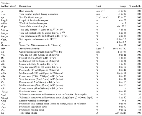
Table 1. List of rain, plot, soil and land use variables used to explain runoff hydrographs; all soil properties were determined for the plough
horizon (approximate depth 0.3 m), if not otherwise indicated. The availability of each variable relative to the total number of runs (n=317) in percent (% available) is also given.
Variable
(Abbreviation) Description Unit Range % available
p Rain intensity mm h−1 31 to 99 100
Ptot Total rainfall applied during simulation mm 31 to 99 100
eP Specific kinetic energy J m−2mm−1 12 to 20 100
length Length of the simulation plot m 4 to 22 100
width Width of the simulation plot m 1 to 2 100
slope Slope of the simulation plot % 1.6 to 23.6 100
CCl_tot Total clay content (<2 µm) in BS(a)(w / w) % 4 to 61 100 CSi_tot Total silt content (2 to 63 µm) in BS (w / w)(b) % 6 to 86 100 CSa_tot Total sand content (63 to 2000 µm) in BS (w / w) % 2 to 87 100
CSOC Soil organic carbon content in FEF(c) % 0.5 to 3.5 100
pH pH – 4.5 to 7.5 80
skeleton Stone (2 to 200 mm) content in BS (w / w) % 0 to 63 100
BD Air-dry bulk density kg m−3 1070 to 1750 42
dg Geometric mean particle diameter(d)of BS µm 1 to 737 100
vfSi Very fine silt (2 to 6.3 µm) in BS (w / w) % 0 to 21 100
fSi Fine silt (6.3 to 20 µm) in BS (w / w) % 1 to 33 100
mSi Medium silt (20 to 36 µm) in BS (w / w) % 1 to 31 100
cSi Coarse silt (36 to 63 µm) in BS (w / w) % 1 to 35 100
vfSa Very fine sand (63 to 100 µm) in BS (w / w) % 0 to 19 100
fSa Fine sand (100 to 200 µm) in BS (w / w) % 0 to 49 100
mSa Medium sand (200 to 630 µm) in BS (w / w) % 0.4 to 61 100
cSa Coarse sand (630 to 2000 µm) in BS (w / w) % 0 to 35 100
vfSt Very fine stones (2 to 6.3 mm) in BS (w / w) % 0 to 31 100
fSt Fine stones (6.3 to 20 mm) in BS (w / w) % 0 to 16 100
mSt Medium stones (20 to 63 mm) in BS (w / w) % 0 to 16 100
cSt Coarse stones (63 to 200 mm) in BS (w / w) % – 100
Fst one Fraction of stone cover % 0 to 35 88
θsurf Volumetric antecedent soil moisture at the surface (0 to 3 cm depth) % 2 to 26 30 θplough Volumetric antecedent soil moisture in the plough layer (0 to 30 cm depth) % 8 to 40 20
Crop Dummy variable of crop type – 0, 1 100
Ftot Fraction of total surface cover (either by stones, plants or residues) % 0 to 93 100
Fveg Fraction of vegetation cover % 0 to 90 88
Fres Fraction of residue cover % 0 to 12 88
tsT Time since tillage d 0.04 to 227 100
(a)Bulk soil;(b)w / w indicates that the soil fractions are calculated relative to the total mass of the soil (kg kg−1);(c)fine earth fraction;(d)according to Sinowski et al. (1995).
most independent variables sufficiently to represent arable landscapes in humid, temperate climate. This is especially true for rain properties, for soil properties and for the distri-bution over seasons. However, the variation in plot dimen-sions is rather limited with a strong collinearity between width and length of the plots, with both restrictions being typical for rainfall simulation experiments.
The simulations were performed through five different re-search groups using different types and set-ups of Veejet noz-zle rainfall simulators. Rainfall intensities varied between 31 and 99 mm h−1, while specific kinetic energy varied from 12 to 20 J m−2mm−1and total rainfall duration varied between
590 and 6180 s. Time to runoff was recorded and plot dis-charge was measured (approx. every minute) by collecting
runoff with calibrated buckets at the lower end of the plots equipped with flow collection gutters (Fiener et al., 2011b).
The data of the different research groups carrying out the simulations had been intensively quality-checked and ho-mogenised into one consistent data set that is freely available (Seibert et al., 2011). Details on the locations, the types of rainfall simulators, plot treatments (e.g. fixed plots vs. mov-ing plots), and measurement conditions used by the different groups are given by Fiener et al. (2011b).
measurements (on average 47 measurements per simulation) used for further analysis.
2.2 Statistical analysis and model development
The selection of any infiltration model makes a fundamen-tal assumption on the underlying runoff generation processes (e.g. crusting vs. infiltration front propagation vs. domi-nance of preferential flow). Following two different and widely used approaches, we fitted Horton-type equations and Green–Ampt-type equations to the hydrographs. Both infiltration equations were flexible enough to be meaning-fully fitted to our data despite their contrasting mechanis-tic justification. Preliminary results showed that both ap-proaches resulted in nearly identical shapes of the hydro-graph and similar efficiencies (R2 was usually above 0.95) and the root mean squared error (RMSE), which was be-low 0.1 mm min−1for both types of equation, was equal to
the unexplained variance in a geostatistical analysis (Fiener at al., 2011b) that does not force any theoretical equation through the data and thus yields the best possible fit. It is important to note that this apparently small error only quan-tifies the random error of multiple runoff rate measurements within an event. Many errors of the infiltration rate apply to all measurements within an event (e.g. errors in plot size or rain intensity; for more details see Fiener et al., 2011b) and potentially cause large errors in the parameters of the infil-tration equations despite a close fit. In consequence, we were not able to decide which process governed runoff generation. Furthermore, we encountered the problem of equifinality (Beven and Binley, 1992); that is, many parameter combina-tions gave statistically similar good results for the same hy-drograph and the same infiltration equation (e.g. the RMSE may only change between 0.032 and 0.035 mm min−1for the same hydrograph, while the initial infiltration rate of the Hor-ton model changed by a factor of three and the decay constant changed by a factor of ten).
Since both approaches yielded identical results and we did not want to decide a priori on a specific modelling philoso-phy, we followed a different, purely statistical approach to estimate surface runoff generation from rainfall plots. We focused on and analysed four support points of the hydro-graphs. These were initial abstraction, defined as rain depth till runoff, and total runoff after 20, 30 and 40 mm of rain (Pa,
QP20, QP30,QP40, respectively; Table 2). Support points
for lower or higher rain depths narrowed the data set and left only subsets which had very early runoff or where high rain depths were applied. Support points for lower or higher rain, hence, were not used at this stage because this reduced the available range of soils, rains and land uses. For the selected four support points, multiple regressions utilising soil, rain and land use variables (Table 1) were developed independently following an iterative approach (e.g. Craw-ley, 2009) taking likely interactions between variables and curvilinear behaviour into account. Given that many
vari-ables correlate (e.g. texture classes but also varivari-ables that were obtained by data transformation) and thus also corre-late similarly to the support points, we chose those variables out of similarly efficient variables that were widely available (e.g. avoiding unusual texture classes), that were meaningful and consistent with current knowledge (e.g. avoiding very narrow texture classes), and that did not produce an unre-alistic behaviour when extended beyond the range covered by measurements (e.g. avoiding transformations that became very steep beyond the measured range). Further, we avoided over-parameterisation by calculating the Bayesian informa-tion criterion (BIC; Kuha, 2004).
Given that some variables were not available for the entire data set (Table 1), such a variable could not be included in the equation developed during one of the successive steps as neither deletion nor imputation of the missing data seemed appropriate. To examine whether such a variable would have had explanatory power, we calculated the residuals between the prediction developed from the entire data set and the mea-sured runoff of the respective subset of data (Framstad et al., 1985). These residuals were then correlated to the omitted variable to examine whether the omitted variable could im-prove the prediction. For example, soil moisture at the very surface or in the plough horizon may likely affect initial ab-straction, but these variables were not available for all hydro-graphs; hence, we developed a prediction equation for initial abstraction without considering soil moisture; then, we cal-culated the residuals of this equation for those hydrographs where the soil moisture was available; these residuals were then correlated with the soil moistures to examine whether soil moisture could explain some of the unexplained varia-tion. None of the other (incomplete) variables had explana-tory power and hence it did not become necessary to consider them in estimating surface runoff.
The selected support points could be predicted using the same soil properties (indicating that dominant influences did not change during the different rainfall events), while only the calibration parameters changed depending on rain depth. Hence, the equations of the selected support points were combined in the next step into one equation, in which the parameterisation depended on rain depth. This equation was then finally fitted to all 14 286 runoff measurements of the 317 hydrographs (approximately 1 min time steps).
2.3 Model and validation
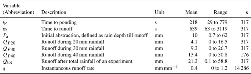
Table 2. Runoff variables from the 317 rainfall simulations used for statistical analysis and model development; the number of available data nvaries according to the availability of the dependent variable.
Variable
(Abbreviation) Description Unit Mean Range n
tP Time to ponding s 218 29 to 779 317
tR Time to runoff s 639 63 to 3119 317
Pa Initial abstraction, defined as rain depth till runoff mm 10 0.7 to 62 317
QP20 Runoff during 20 mm rainfall mm 4.1 0 to 16.5 317
QP30 Runoff during 30 mm rainfall mm 9.3 0 to 26.7 317
QP40 Runoff during 40 mm rainfall mm 13.4 0 to 30.8 176
Qtot Runoff after total rainfall of an experiment mm 21.3 0.1 to 58.8 317
q Instantaneous runoff rate mm mm−1 0.4 0 to 1.2 14 286
validation. This procedure was repeated ten times assuring that every hydrograph was used once for validation. The ten folds yielded a family of similar equations for all subsets that satisfactorily predicted the validation data (see Results).
Finally, we compared the quality of our predictions with predictions derived following the classical curve number (CN) approach (Mockus, 1972), which is the most prominent statistical approach to estimate surface runoff. The hydrolog-ical soil groups of the CN approach were assigned based on the soil descriptions (not based entirely on topsoil properties as recorded in the database). For fallow, row crop and small grain a low runoff disposition was always assumed. Fur-thermore, CNs were estimated with an alternative approach following Auerswald and Haider (1996) using soil cover of row crops and small grains, respectively. The second CN ap-proach was developed using a subset of the data set used in this study (Auerswald and Haider, 1996).
All statistical analyses were carried out using the GNU R version 2.14.0 (R Development Core Team, 2011). Be-sidesR2 and RMSE we also used the Nash–Sutcliffe effi-ciency (NSE; Nash and Sutcliffe, 1970) as a goodness of fit parameter.
3 Results
3.1 Support points
The initial abstractionParanged from 0.7 to 62 mm for the
317 hydrographs, but only two of the variables contributed to the explanation of this variation. These were total stone cover exceeding 10 %Fstone>10 % (range 0 to 25 %), which
was calculated asFstone>10 %= max (0;Fstone–10), and sand
content (0.063 to 2 mm) of the bulk soilCSa_tot(range 2 to
87 %). With increasing stone cover, time to runoff (and hence initial abstraction) increased, while increasing sand content promoted earlier runoff (Eq. 1):
Pa=16.2+1.37×Fstone>10 %−2.52×ln(CSa_tot). (1)
Equation (1) explained 53 % of the variation (RMSE 6 mm) ofPa, whileFstone>10 %andCSa_totexplained 37 and 10 mm
of the variation, respectively. The RMSE was rather large (andR2low), indicating that initial abstraction was strongly influenced by factors that could not be captured by the avail-able variavail-ables. Remarkably, rain intensity, which spanned from 29 to 99 mm h−1, had no influence on initial abstraction (R2=0.0002), while it dominated the time to runoff because initial abstraction was reached earlier with increasing rain in-tensity. Also, soil moisture in the surface soil (0.03 m; range: 2 to 26 w / %) or in the plough layer (range: 8 to 40 w / w-%), which both may especially influence early runoff, did not improve the prediction ofPa.
QP20,QP30andQP40were all explained best by the same
variables, namely rain intensity, time since tillage and or-ganic carbon content. This lead to equations of the following type:
QP=f+g×(p)−h×ln(tsT)+k×ln(tsT)4+l×ln(CSOC), (2)
where QP is the accumulated runoff volume (mm) since
the start of rain to rain depth P (mm); p is rain intensity (mm h−1);tsT is time since tillage (d);CSOC is soil carbon
content (%); andf,g,h,k andl are empirical parameters that vary with rain depthP.
In general, the higherpwas, the more runoff was observed after a given rain depth because the time available for infil-tration decreased. The strongest influence, however, was ex-hibited bytsT, which usually is not regarded in hydrological
modelling. With increasingtsT runoff decreased. For
exam-ple, runoff after 30 mm of rain was on average 20 mm if the rainfall occurred within less than an hour after tillage, while it was less than 5 mm if the rainfall occurred more than 100 days after tillage. This effect was particularly pronounced for shorttsT (in the range of few hours to single days) although
it lasted even for more than 200 days. This strongly decreas-ing effect made it necessary to use the logarithm and to use a second term (ln(tsT)4)in Eq. (2), which compensates some of
the term (ln(tsT))at hightsT. IncreasingCSOCalso decreased
-20 -10 0 10 20
0.00 0.05 0.10 0.15 0.20
ErrorQ(mm)
Density
-1 -0.5 0 0.5 1
0.0 0.5 1.0 1.5 2.0 2.5
Errorq(mm mm-1)
[image:6.595.48.284.60.176.2]Density
Fig. 1. Error distribution of accumulated runoff depthQand instan-taneous runoff rateq for 14 286 runoff measurements during 317 events.
large number of available explanatory variables (Table 1) and the large number of measurements, no further variable im-proved the runoff prediction. This was especially true for soil physical properties that are commonly assumed to influence runoff (e.g. texture variables, porosity, and moisture).
3.2 Hydrograph prediction
Given the identical behaviour of all support points, the parameters of Eq. (2) could be optimised for any rain depth P by using all data. The best combination of parameters was d=2.6 mm, e=3.3 mm ln(mm)−1, f=
0.6, g=4.3×10⁻³h mm−1, h=7.6×10⁻² ln(d)−1, k=
5.0 ×10⁻⁶ln(d)−4, andl=0.19 ln(%)−1for the final equa-tion:
QPr=d−e×ln(Pr)+Pr×f+g×p−h × ln(tsT)+k× ln(tsT)4−l
× ln(CSOC)] (3)
for Pr> e/f+g×p−h
× ln(tsT)+k×ln(tsT)4−l×ln(CSOC) i
and QPr>0 else QPr=0,
whereQPris runoff volume (mm) at rain depthPr(mm)
ex-ceeding initial abstraction given byPr=P−Pa.
The combining of Eqs. (1) and (3) allowed the computa-tion of hydrographs for all 317 events. The calculated hy-drographs explained 72 % of the variability of the measured accumulated runoff volumes (RMSE 5.2 mm; NSE 0.71), as compared to 58 % of the variation in instantaneous runoff rates (RMSE 0.23 mm mm−1; NSE 0.56). The error
distri-butions (Fig. 1) showed a pronounced excess kurtosis, in-dicating that the errors were usually less than half as indi-cated by the RMSEs with the exception of some hydrographs that were poorly predictable. We checked these hydrographs and the corresponding experimental descriptions but found no anomalies that could explain the behaviour of these hy-drographs. It is important to note that RMSEs also account for sampling errors associated with field measurements and
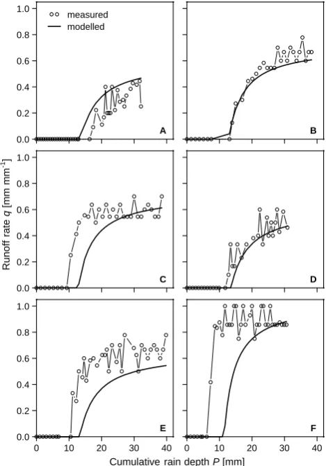
0.0 0.2 0.4 0.6 0.8 1.0
measured modelled
A B
0.0 0.2 0.4 0.6 0.8 1.0
C
Runoff
rate
q
[mm
m
m
-1]
D
0 10 20 30 40
0.0 0.2 0.4 0.6 0.8 1.0
Cumulative rain depthP[mm] E
0 10 20 30 40
[image:6.595.311.546.63.399.2]F
Fig. 2. Examples of instantaneous runoff rates during six events in
different months and years on one plot kept under seedbed condi-tions. Note: time since tillage is 0.04 day in panel F, while it is∼3–5 days in all other cases.
for inconsistencies among research groups that contributed to the combined data set. The measured instantaneous runoff rates per minute are subject to random errors that level out when rates over a longer period of time are combined in the calculation of the accumulated runoff volume, while system-atic errors (bias) of the rate measurements also affect runoff volume. The difference in performance of rates and volume thus was due to the influence of random error. The random error in measured runoff rates along a single hydrograph typically was ±0.1 mm mm−1 (Fig. 2) or half of the over-all RMSE. No model can capture such random errors and also the biases, which are even more difficult to identify (e.g. errors in plot size determination). It is hence unlikely that another equation could explain the hydrographs better.
0 50 100 150 200 0 5 10 15 20 25 30 35
tsT[d]
20 mm 30 mm 40 mm 50 mm 60 mm
0.5 1 1.5 2 2.5 3 3.5 0 5 10 15 20 25 30 35
CSOC[%] Modelled
runoff v olume QP20 to P 60 [mm]
30 40 50 60 70 80 90 100 0 5 10 15 20 25 30 35
p[mm h-1]
Rainfall depths
0 20 40 60 80 0 5 10 15 20 25 30 35
cSa_tot[%]
0 5 10 15 20 25 30 35 0 5 10 15 20 25 30 35
Fstone[%]
[image:7.595.50.280.63.391.2]Modelled runoff v olume QP20 to P 60 [mm]
Fig. 3. Modelled accumulated runoff volumes (QP20 to 60)for
dif-ferent rainfall depths (20 to 60 mm) and varying total sand content
CSa_tot, stone coverFstone, time since tillagetsT, soil organic
car-bon contentCSOC, and rainfall intensitypas used in Eqs. (1) and
(3); for the modelling approach all variables except the one varied were kept constant at their mean value (for values see Fig. 4).
of tsT as this hydrograph was obtained only one hour
af-ter tillage, while the other hydrographs were obtained 3 to 5 days after tillage. Despite near-constant soil, plot and rain properties for some of the other hydrographs (e.g. D and E, except for the fact that more rain was applied in the case of E), there were differences for which no explanation ex-ists and which hence can also not be captured by the model. Despite this, the model with only five variables explained all hydrographs reasonably well even though three variables (Fstone>10 %,CSa_tot, andCSOC)were held constant because
they were determined only once on this plot.
The sensitivities of the variables within the complete model were analysed by changing the values of each vari-able within its measured range (Tvari-able 1), while rainfall depth increased from 0 to 60 mm and the other variables were held constant at their mean values (Figs. 3 and 4). With increas-ing sand content, runoff started earlier (Fig. 4), but the ef-fect was small and most prominent for small sand contents (approximately 0 to 10 %; Fig. 3). Stone cover had a much
CSa_tot[%]
Fstone[%]
tsT[d]
CSOC[%]
p[mm h-1]
87 87 28 2 28 2 0(= 6.6) 35 35 0 10 20 30 40 50 0.0 0.2 0.4 0.6 0.8 1.0
0 20 40 60 0 10 20 30 40 50
0 20 40 60 0.0 0.2 0.4 0.6 0.8 1.0
Cumulative rainfallP[mm]
0 10 20 30 40 50 0.0 0.2 0.4 0.6 0.8 1.0 0 10 20 30 40 50 0.0 0.2 0.4 0.6 0.8 1.0 0 10 20 30 40 50 Runoff v ol ume Q [mm] 0.0 0.2 0.4 0.6 0.8 1.0 Runoff rate q [mm m m -1] 0.04 12 227 0.04 12 227 0.5 1.4 3.5 0.5 1.4 3.5 99 61 31 99 61 31
[image:7.595.310.547.83.584.2]0 (= 6.6)
Fig. 4. Modelled accumulated runoff volume (left column) and
in-stantaneous runoff rate (right column) for mean (bold line), min-imum (dotted line), and maxmin-imum (thin line) values of total sand contentCSa_tot, stone coverFstone, time since tillagetsT, soil
or-ganic carbon contentCSOC, and rainfall intensityp. Numbers
de-note the minimum, mean and maximum of each variable. All vari-ables were kept constant at their mean value except the one varied. ForFstonethe minimum and the mean result in the same hydrograph
Table 3. Calibration and validation results of accumulated runoff
volumes (Q)and instantaneous runoff rates (q)for all 317 hydro-graphs used in a ten-fold cross validation; Goodness-of-fit param-eters were calculated based on the full model/data resolution of 1 min; NSE is Nash–Sutcliffe efficiency (Nash and Sutcliffe, 1970),
R2is the coefficient of determination, and RMSE is the root mean square error;nindicates the number of single measurements used for calibration and validation.
Q[mm] q[mm mm−1]
Calibration Validation Calibration Validation
n 128 574 14 286 128 574 14 286
R2 0.72 0.72 0.58 0.58
RMSE 5.19 5.21 0.23 0.23
NSE 0.71 0.71 0.56 0.55
larger effect on runoff initiation and hence on runoff depths (Figs. 3 and 4). Increasing stone cover increasingly retarded runoff, but this became effective only above a threshold of 10 % stones (Fig. 3). Consequently, stone cover can be ne-glected for many soils because the average stone cover in our data set was 6.6 %. Importantly, sand content and stone cover influenced the whole hydrograph (Fig. 4) beyond the start of runoff due to the fact that Eq. (1) was needed to calculate Eq. (3).
With increasing rainfall intensity, instantaneous runoff rates and accumulated volumes increased as predicted by Eq. (3). This also influenced the start of runoff. Runoff started slightly later with decreasing rain intensity (Fig. 4) even though intensity was not part of Eq. (1). This is because the influence of intensity on initial abstraction was rather weak when compared to the random scatter of initial abstrac-tion. Using all runoff measurements, as in Eq. (3), instead of using only one data point (initial abstraction) reduced the random scatter, and thus this influence became visible in the final Eq. (3). Thus, Eq. (1) was not sufficient to calculate the start of runoff and so was used as an intermediate step in the development of Eq. (3). The same behaviour was true for all other variables that additionally entered Eq. (3).
The influence ofCSOCwas of similar strength as rainfall
intensity. Instantaneous runoff rates and accumulated vol-umes decreased with increasingCSOC (Fig. 3) and caused
the runoff to start later (Fig. 4). The time since tillage tsT
effect was about 30 % stronger thanCSOCand rainfall
inten-sity (compare final ranges of runoff volume and rate), but this was an effect of the very shorttsT(minimum: 1 h) that were
possible with small plots and artificial rainfall but which will unlikely occur on larger fields that need considerably longer than 1 h for tillage. Considering the range of time relevant for whole fields, the influence oftsT was similar in strength to
the other influences. The change during the first 12 days af-ter tillage was about the same as the change occurring during the following 215 days (Fig. 4).
0 10 20 30 40 50 60
0 10 20 30 40 50 60
Pa
0 10 20 30 40 50 60
0 10 20 30 40 50 60
QP20
0
0 10 20 30 40 50 60 0
10 20 30 40 50 60
MeasuredPa,QP20,QP30,QP40[mm]
Modelled
Pa
,
QP2
0
,
QP3
0
,
QP4
0
[mm]
QP30
0 10 20 30 40 50 60 0 10 20 30 40 50 60
Modelled
Pa
,
QP2
0
,
QP3
0
,
QP4
0
[mm]
[image:8.595.48.286.158.243.2]QP40
Fig. 5. Modelled vs. measured initial abstractionPa, and
accumu-lated runoff after 20, 30 and 40 mm of rainfall (QP20,QP30 and
QP40, respect ively); data shown combine all validation results of
the ten-fold cross validation; root mean square errors are 7.0, 3.5, 5.3, and 6.9 forPa,QP20,QP30, andQP40, respectively.
3.3 Model validation
The restricted data sets of the folds created during cross val-idation led to models similar to those using the full data set. The prediction quality did not differ between the calibration and the validation data sets for both runoff volume and rate (Table 3), indicating that all models were equally suitable for predictions. The models explained the validation data with a NSE between 0.55 and 0.71 (Table 3, Fig. 5). Runoff volume again was modelled more accurately than runoff rate. Runoff varied between 0 and 59 mm and could be predicted with RMSE=5.2 mm. However, the models performed somewhat weaker for initial abstraction, as mentioned earlier, since
Pa is strongly influenced by factors that could not be
cap-tured with the available variables. In general, prediction qual-ity increased with rainfall volume and hence surface runoff volume (Fig. 5).
4 Discussion
4.1 Initial abstraction
In general, initial abstraction showed substantially more ran-dom (unexplained) variability than subsequent runoff rates, indicating that these measurements are more prone to un-certainty. The high variability of initial abstraction under more or less identical plot conditions could have resulted from small random differences; e.g. compaction at the down-slope end of the plot will encourage early runoff or small depressions at the outlet will increase detention storage and hence delay first runoff. Such random differences are likely to occur given that most of the plots were situated in ordi-nary farmed fields. Also subjective decisions by the technical staff carrying out the rainfall simulations are necessary when recording the first runoff (whether it starts with the first sin-gle drop or the first continuous flow). These decisions will differ among research groups contributing the data, persons within a group and even for the same person during differ-ent measuring campaigns. Hence, when initial abstraction was analysed without consideration of the following runoff measurements, it was best explained by the combination of only two soil properties, namelyFstone>10 % and sand
con-tent (Eq. 1), despite its large variability (Table 2). However, all other variables which influenced the hydrograph also af-fected initial abstraction (Fig. 4) because (at the plot scale) abstraction must become larger the slower the hydrograph rises. The effect ofFstone>10 % most probably resulted from
the macropore space under stones created during tillage that can store runoff. The threshold indicated that small stone contents, which usually also are associated with small and rounded stones, did not exhibit this effect. In this case it can be expected that the small stones are embedded within the soil matrix and may even decrease infiltration rates (Wilcox et al., 1988). This threshold agrees with the calculation of soil erodibility in the revised universal soil loss equation, which also uses a threshold of 10 % for the consideration of stones (Roemkens et al., 1997). Also Poesen et al. (1994) suggested this threshold. In general, the importance of the variable
Fstone>10 % is in line with findings of Poesen et al. (1990),
indicating that stones not fully embedded in the surface soil layer typically lead to preferential infiltration of runoff under these stones, and with Tromble (1976), who found a positive relation between infiltration and stone cover after ploughing rangeland. Even though the influence of stones on initial ab-straction was large, this applied only for a small number of soils. Only 36 % of our soils had a stone cover just above the threshold and only 16 % were above a stone cover of
>15 %. For the USA it was estimated that stones need to be considered in the calculation of soil erodibility on 16 % of the land area (Roemkens et al., 1997). Similar percent-ages may hence be found in many temperate areas of the world, while in other areas like the Mediterranean stony soils may even occupy much larger areas (60 % according to
Poe-sen and Lavee, 1994) and cause the low erosion rates there (Cerdan et al., 2011).
The influence of sand content was opposite to what might be expected (e.g. from the influence of texture in the SCS CN model) although our model is still in general agreement with the assessment of coarse-textured soils by the CN model due to the fact that stones had a much larger influence than sand and because the CN model does not explicitly distinguish be-tween the effects of stones and sand. There is little systematic research on the effect of sand on runoff, which impedes the interpretation of this result. It is remarkable, however, that the influence of sand only promoted early runoff but not later runoff (Figs. 3, 4). Likely, the increasing sand content de-creased aggregate stability (Boix-Fayos et al., 2001) and in-creased slaking forces (Auerswald, 1995) due to the usually dry soil surface of sandy soils. Both promote the breakdown of aggregates and thus accelerate sealing and decrease de-pression storage on the soil surface (Mohamoud et al., 1990).
4.2 Hydrograph shape
The hydrographs could be predicted surprisingly well with an interaction of simple rain, soil and land-use variables despite the large variation in the data set. These were rain depth ex-ceeding initial abstraction, rain intensity, soil organic carbon content and time since tillage. The importance of rain depth exceeding initial abstraction and rain intensity is obvious and is also important in many other surface runoff estimates (e.g. Appels et al., 2011).
The influence ofCSOCon hydraulic parameters (e.g.
Ra-jkai et al., 2004; Scheinost et al., 1997) and erosion (Guerra, 1994) has been shown in several studies. Its influence on the hydrograph likely results from (i) a larger aggregate stabil-ity (Auerswald, 1995; Tisdall and Oades, 1982), (ii) larger unsaturated hydraulic conductivity, and (iii) higher biologi-cal activity (e.g. Anderson and Domsch, 1989; Weigand et al., 1995) especially by earthworms creating more voids for runoff intake (Auerswald et al., 1996). It is important to note that the soils for which these relationships have been specif-ically quantified by Weigand et al. (1995) and Auerswald et al. (1995, 1996) comprise a large portion of the present data set. It is thus likely that biological activity, earthworm abun-dance and cross-sectional area of biopores, which were avail-able for these soils, would have been good predictors for the entire data set if they had been available for all runs. How-ever, given that these variables are usually not available for prediction,CSOCis preferable even though it may only
influ-ence infiltration indirectly via aggregate stability and biopore cross-sectional area.
More difficult to interpret is the importance oftsT, because
and Connolly, 1995; Choudhary et al., 1995) and thus ac-knowledge the prominent impact of tillage on runoff. How-ever, these comparisons are usually done between treatments, while the changes over time are hardly considered although tillage impacts many physical and biological soil properties, which then gradually change until the next tillage (Caron et al., 1992; Dexter et al., 1998; Franzluebbers et al., 1995; Zobeck and Onstad 1987). Surface runoff decreased with in-creasingtsT, while the opposite might be expected from the
typically observed decrease in porosity following a number of drying–wetting cycles after tillage (Ahuja et al., 2006; Franzluebbers et al., 1995; Onstad, 1984) and the decrease in detention and depression storage due to a decrease in ran-dom roughness with consecutive rainfalls (Zobeck and On-stad, 1987). Several processes likely contribute at different time scales as tsT covered nearly four magnitudes (1 h to
227 days; Table 1). (i) In the short term (several hours af-ter tillage) the fast drying of freshly tilled soil can increase infiltration capacity and stabilise aggregates during drying (Crouch and Novruzi, 1989; Gollany et al., 1991). The lat-ter reduces soil crusting potential and promotes infiltration. (ii) Within several days following tillage, age hardening of the aggregates will take place due to drying (cycles) and due to biological activity. Biological activity produces bind-ing substances, includbind-ing hyphae that form more and closer bonds between soil particles, causing cementing substances to precipitate at newly formed particle contacts (Dexter et al., 1988; Kemper and Rosenau, 1984; Schweikle et al., 1974). All of these mid-term processes of soil structure stabilisa-tion potentially prevent soil crusting, which is most important shortly after tillage since soils are not fully covered by grow-ing crops. (iii) In the long run (weeks to months),tsTis
prob-ably also a proxy for the development of plant cover, includ-ing changes in tilth underneath a cover and the development of connected biopores reaching the soil surface, even though none of the four cover variables (Table 1) entered any equa-tion. These interpretations have to remain speculative given the little attentiontsThas previously attained in runoff
stud-ies. To our knowledge, this parameter has only be analysed in respect to aggregate stability and soil erosion, where it can exhibit a large effect (e.g. Auerswald, 1993; Auerswald et al., 1994; Caron et al., 1992; Shainberg et al., 1996), but not for runoff generation. Typically this information is not reported in publications, which may explain the often large difference in runoff between different studies as well as some of the unexplained scatter within individual studies given the large changes that can happen at shorttsT. More attention should
be paid to variables related to tillage practices given the fact that seedbed conditions, which fall into this range, are often analysed.
It is remarkable that the CN approach by Auerswald and Haider (1996) did not perform better than the original version by Mockus (1972) although Auerswald and Haider (1996) had used a subset of our data to develop their equation, which predicts CN from soil cover. Within their subset of data, soil
cover mainly changed due to early plant growth and hence it had statistically a similar power totsT. For the entire data set,
tsT was superior to soil cover because it also described the
changes immediately after tillage before the onset of plant growth. Additionally, tsT can also serve as an indicator for
long-term changes, while soil cover approaches its final value usually two months after seeding.
It is debatable whether any empirical or mechanistic ap-proach to model surface runoff generation can be reliably transferred to other sites given the multitude of conceivable influences. As our data set covers a large range of rainfall, topography, soil and land-use properties (Table 1) the re-sults from the validation are encouraging for our statistical approach. The overall RMSE of accumulated runoff volume and instantaneous runoff rate of 5.2 mm and 0.23 mm mm−1, respectively, probably cannot be lowered markedly by an-other model predicting rain excess and runoff generation be-cause such differences already existed in the data measured in replicated plots (Fig. 2). The differences must be caused either by systematic measuring errors like a wrong rain inten-sity or by properties that were not measured, and thus would not be available for other types of models (e.g. antecedent sealing, biopore density, biopore connectivity etc.).
5 Conclusions
The large data set of 317 rainfall simulations (14 286 runoff measurements) represented a wide range of arable soils and crops. Runoff measurements were related to 20 time-invariant soil properties, three variable soil properties, four rain properties, three land use properties and derived vari-ables. In an iterative multiple regression procedure six of these properties/variables best described initial abstraction and the hydrograph. The fraction of stone cover above 10 %
Fstone>10 %and the content of total sand in the fine earth
frac-tionCSa_totwere needed to estimate initial abstraction, while
the hydrograph could be predicted from rain depth exceeding initial abstractionPr, rainfall intensityp, soil organic matter
contentCSOC, and time since last tillage tsT. The resulting
model predicted event hydrographs without a priori assump-tions of the underlying process (e.g. Hortonian vs. satura-tion runoff generasatura-tion). Validating this approach by creating a family of models by ten-fold cross validation indicated that these models explained 72 % of variability in runoff volume and 58 % of runoff rate (RSME: 5.2 mm and 0.23 mm mm−1,
respectively) of the training data and also of the validation data. It outperformed the CN approach, and thus implementa-tion in spatially distributed and temporally continuous mod-els that capture agricultural management seems promising.
Stone cover was most important for the initial abstrac-tion, whiletsTwas most important for the hydrograph. These
approaches to address infiltration. This finding should foster a discussion regarding our ability to accurately model sur-face runoff from arable land, which seemed to be dominated by agricultural operations introducing a man-made seasonal-ity to soil hydraulic properties.
Acknowledgements. We gratefully acknowledge the work and
efforts of all research groups collecting the data set used in this meta-analysis, especially K. Gerlinger, J. Haider, W. Martin, and A. Michael. S. P. Seibert compiled the data set and ran extensive preliminary analyses. R. Quinones provided linguistic help. This research was conducted within the German Research Agency (DFG) project DI 639/2-1; the financial support by the DFG is acknowledged.
Edited by: D. Mazvimavi
References
Ahuja, L. R., Ma, L., and Timlin, D. J.: Trans-disciplinary soil physics research critical to synthesis and modeling of agricul-tural systems, Soil Sci. Soc. Am. J., 70, 311–326, 2006. Anderson, T. H. and Domsch, K. H.: Ratios of microbial biomass
carbon to total organic carbon in arable soils, Soil Biol. Biochem., 21, 471–479, 1989.
Appels, W. M., Bogaart, P. W., and van der Zee, S. E. A. T.: In-fluence of spatial variations of microtopography and infiltration on surface runoff and field scale hydrological connectivity, Adv. Water Resour., 34, 303–313, 2011.
Assouline, S. and Mualem, Y.: Runoff from heterogeneous small bare catchments during soil surface sealing, Water Resour. Res., 42, W12405, doi:10.1029/2005WR004592, 2006.
Auerswald, K.: Influence of initial moisture and time since tillage on surface structure breakdown and erosion of a loessial soil, Catena Suppl, 24, 93–101, 1993.
Auerswald, K.: Percolation stability of aggregates from arable top-soils, Soil Sci., 159, 142–148, 1995.
Auerswald, K. and Haider, J.: Runoff curve numbers for small grain under German cropping conditions, J. Environ. Manage., 47, 223–228, 1996.
Auerswald, K., Mutchler, C. K., and McGregor, K. C.: The influ-ence of tillage-induced differinflu-ences in surface moisture content on soil erosion, Soil Tillage Res., 32, 41–50, 1994.
Auerswald, K., Weigand, S., Kainz, M., and Philipp, C.: Influence of soil properties on the population and activity of geophagous earthworms after five years of bare fallow, Biol. Fertil. Soils, 23, 382–387, 1996.
Beven, K. and Binley, A.: The future of distributed models: model calibration and uncertainty prediction, Hydrol. Process., 6, 279– 298, 1992.
Boix-Fayos, C., Calvo-Cases, A., Imeson, A. C., and Soriano-Soto, M. D.: Influence of soil properties on the aggregation of some Mediterranean soils and the use of aggregate size and stability as land degradation indicators, Catena, 44, 47–67, 2001.
Borah, D. K. and Bera, M.: Watershed-scale hydrologic and nonpoint-source pollution models: Review of mathematical bases, T. ASAE, 46, 1553–1566, 2003.
Caron, J., Kay, B. D., Stone, J. A., and Kachanoski, R. G.: Modeling temporal changes in structural stability of a clay loam soil, Soil Sci. Soc. Am. J., 56, 1597–1604, 1992.
Cerdan, O., Govers, G., Le Bissonnais, Y., Van Oost, K., Poesen, J., Saby, N., Gobin, A., Vacca, A., Quinton, J., Auerswald, K., Klik, A., Kwaad, F. J. P. M., Raclot, D., Ionita, I., Rejman, J., Rous-seva, S., Muxart, T., Roxo, M. J., and Dostal, T.: Rates and spatial variations of soil erosion in Europe: a study based on erosion plot data, Geomorphology, 122, 167–177, 2010.
Choudhary, M. A., Lal, R., and Dick, W. A.: Long-term tillage ef-fects on runoff and soil erosion under simulated rainfall for a central Ohio soil, Soil Tillage Res., 42, 175–184, 1997. Crawley, M. J.: The R Book. Wiley, Chichester, UK, 2009. Crouch, R. J. and Novruzi, T.: Threshold conditions for rill initiation
on a Vertisol, Gunnedah, N. S. W., Australia. Catena, 16, 101– 110, 1989.
Dexter, A. R., Horn, R., and Kemper, W. D.: Two mechanisms for age-hardening of soil, J. Soil Sci., 39, 163–175, 1988.
EUROSTAT: Land cover and land use overview by NUTS 1 regions, available at: http://appsso.eurostat.ec.europa.eu/nui/ setupModifyTableLayout.do (last access: 8 November 2012), 2012.
Evrard, O., Vandaele, K., Bielders, C., and Van Wesemael, B.: Sea-sonal evolution of runoff generation on agricultural land in the Belgian loess belt and implications for muddy flood triggering, Earth Surf. Proc. Landf., 33, 1285–1301, 2008.
Fiener, P., Govers, G., and Van Oost, K.: Evaluation of a dynamic multi-class sediment transport model in a catchment under soil-conservation agriculture, Earth Surf. Proc. Landf., 33, 1639– 1660, 2008.
Fiener, P., Auerswald, K., and Van Oost, K.: Spatio-temporal pat-terns in land use and management affecting surface runoff re-sponse of agricultural catchments – a review, Earth-Sci. Rev., 106, 92–104, 2011a.
Fiener, P., Seibert, S. P., and Auerswald, K.: A compilation and meta-analysis of rainfall simulation data on arable soils, J. Hy-drol., 409, 395–406, 2011b.
Framstad, E., Engen, S., and Stenseth, N. C.: Regression analy-sis, residual analysis and missing variables in regression models, Oikos, 44, 319–323, 1985.
Franzluebbers, A. J., Hons, F. M., and Zuberer, D. A.: Tillage-induced seasonal changes in soil physical properties affecting soil CO2evolution under intensive cropping, Soil Tillage Res.,
34, 41–60, 1995.
Gollany, H. T., Schumacher, T. E., Evenson, P. D., Lindstrom, M. J., and Lemme, G. D.: Aggregate stability of an eroded and desur-faced Typic Argiustoll, Soil Sci. Soc. Am. J., 55, 811–816, 1991. Green, T. R., Ahuja, L. R., and Benjamin, J. G.: Advances and chal-lenges in predicting agricultural management effects on soil hy-draulic properties, Geoderma, 116, 3–27, 2003.
Green, W. H. and Ampt. G. A.: Studies on soil physics. 1. Flow of air and water through soils, J. Agr. Sci., 4, 1–24, 1911.
Guerra, A.: The effect of organic matter content on soil erosion in simulated rainfall experiments in W. Sussex, UK, Soil Use Man-age., 10, 60–64, 1994.
Haygarth, P. M., Bilotta, G. S., Bol, R., Brazier, R. E., Butler, P. J., Freer, J., Gimbert, L. J., Granger, S. J., Krueger, T., Macleod, C. J. A., Naden, P., Old, G., Quinton, J. N., Smith, B., and Worsfold, P.: Processes affecting transfer of sediment and colloids, with associated phosphorus, from intensively farmed grasslands: An overview of key issues, Hydrol. Process., 20, 4407–4413, 2006. Horton, R. E.: An approach toward a physical interpretation of
in-filtration capacity, Soil Sci. Soc. Am. J., 5, 399–417, 1940. Kale, R. V. and Sahoo, B.: Green-Ampt infiltration models for
var-ied field conditions: A revisit, Water Resour. Manage., 25, 3505– 3536, 2011.
Kemper, W. and Rosenau, R.: Soil cohesion as affected by time and water content, Soil Sci. Soc. Am. J., 48, 1001–1006, 1984. Klar, C., Fiener, P., Lenz, V., Neuhaus, P., and Schneider, K.:
Mod-elling of soil nitrogen dynamics within the decision support sys-tem DANUBIA, Ecol. Modell., 217, 181–196, 2008.
Kohavi, R.: A study of cross-validation and bootstrap for accuracy estimation and model selection. Proceedings of the Fourteenth International Joint Conference on Artificial Intelligence 2, Mor-gan Kaufmann, San Mateo, CA, 1137–1143, 1995.
Kuha, J.: AIC and VIS – Comparisons of assumptions and perfor-mance, Sociol. Meth. Res., 33, 188–229, 2004.
Li, H., Sivapalan, M., and Tian, F.: Comparative diagnostic analysis of runoff generation processes in Oklahoma DMIP2 basins: The Blue River and the Illinois River, J. Hydrol., 418–419, 90–109, 2012.
Migliaccio, K. W. and Srivastava, P.: Hydrologic components of watershed-scale models, T. ASABE, 50, 1695–1703, 2007. Mockus, V.: Estimation of direct runoff from storm rainfall. SCS
National Engineering Handbook. Section 4, Hydrology 10.1– 10.24 USDA, Washington D.C., USA, 1972.
Mohamoud, Y. M., Ewing, L. K., and Boast, C. W.: Small plot hy-drology: I. Rainfall infiltration and depression storage determi-nation, T. ASAE, 33, 1121–1131, 1990.
Nahar, N., Govindaraju, R. S., Corradini, C., and Morbielli, R.: Nu-merical evaluation of the role of runon on sediment transport over heterogeneous hillslopes, J. Hydrol. Eng., 13, 215–225, 2008. Nash, J. E. and Sutcliffe, J. V.: River flow forecasting through
con-ceptual models: Part I. A discussion of principles, J. Hydrol., 10, 282–290, 1970.
Onstad, C. A.: Effect of rainfall on tilled soil properties, Am. Soc. Agr. Eng. Paper, No. 84–2525, 1984.
Philip, J. R.: Theory of infiltration, Adv. Hydrosci., 5, 215–296, 1969.
Poesen J. W. and Lavee H.: Rock fragments in top soils: Signifi-cance and processes, Catena, 23, 1–28, 1994.
Poesen, J., Ingelmo-Sanchez, F., and Mücher, H.: The hydrologi-cal response of soil surfaces to rainfall as affected by cover and position of rock fragments in the top layer, Earth Surf. Process. Landf., 15, 653–671, 1990.
Poesen, J. W., Torri, D., and Bunte K.: Effects of rock fragments on soil erosion by water at different spatial scales: A review, Catena, 23, 141–166, 1994.
R Development Core Team. R: A language and environment for statistical computing, available at: http://www.R-project.org (last access: March 2013), R Foundation for Statistical Computing, 2011.
Rajkai, K., Kabos, S., and Van Genuchten, M. T.: Estimating the water retention curve from soil properties: Comparison of linear, nonlinear and concomitant variable methods, Soil Tillage Res., 79, 145–152, 2004.
Römkens, M. J. M., Young, R. A., Poesen, J. W. A., McCool, D. K., El-Swaify, S. A., and Bradford, J. M.: Soil erodibility factor (K), in: Predicting Soil Erosion by Water: A Guide to Conser-vation, edited by: Renard, K. G., Foster, G. R., Weesies, G. A., McCool, D. K., and Yoder, D. C., coordinators, Planning with the Revised Universal Soil Loss Equation (RUSLE), US Department of Agriculture, Agriculture Handbook No. 703, 65–99, 1997. Scheinost, A. C., Sinowski, W., and Auerswald, K.: Regionalization
of soil water retention curves in a highly variable soilscape, I. De-veloping a new pedotransfer function, Geoderma, 78, 129–143, 1997.
Schweikle, V., Blake, G. R., and Arya, L. M.: Matric suction and stability changes in sheared soils, Trans 10th Inter Congress Soil. Sci. I, 187–193, 1974.
Seibert, S. P., Auerswald, K., Fiener, P., Disse, M., Martin, W., Haider, J., Michael, A, and Gerlinger, K. Surface runoff from arable land – a homogenized data base of 726 rainfall simulation experiments, doi:10.1594/GFZ.TR32.2, 2011.
Shainberg, I., Goldstein, D., and Levy, G. J.: Rill erosion depen-dence on soil water content, aging, and temperature, Soil Sci. Soc. Am. J., 60, 916–922, 1996.
Silburn, D. M. and Connolly, R. D.: Distributed parameter hydrol-ogy model (ANSWERS) applied to a range of catchment scales using rainfall simulator data I: Infiltration modelling and param-eter measurement, J. Hydrol., 172, 87–104, 1995.
Sinowski, W.: Die dreidimensionale Variabilität von Bodeneigen-schaften – Ausmaß, Ursachen und Interpolation. Shaker, Aachen, Germany, 1995.
Smith, M. B., Seo, D. J., Koren, V. I., Reed, S. M., Zhang, Z., Duan, Q., Moreda, F., and Cong, S.: The distributed model intercom-parison project (DMIP): motivation and experiment design, J. Hydrol., 298, 4–26, 2004.
Tian, F. Q., Li, H. Y., and Sivapalan, M.: Model diagnostic analysis of seasonal switching of runoff generation mechanisms in the Blue River basin, Oklahoma, J. Hydrol., 418, 136–149, 2012. Tisdall, J. M. and Oades, J. M.: Organic matter and water-stable
aggregates in soils, J. Soil Sci., 33, 141–163, 1982.
Tromble, J. M.: Semiarid rangeland treatment and surface runoff, J. Range Manage., 29, 251–255, 1976.
Vivoni, E. R., Entekhabi, D., Bras, R. L., and Ivanov, V. Y.: Con-trols on runoff generation and scale-dependence in a distributed hydrologic model, Hydrol. Earth Syst. Sci., 11, 1683–1701, doi:10.5194/hess-11-1683-2007, 2007.
Weigand, S., Auerswald, K., and Beck, T.: Microbial biomass in agricultural topsoils after six years of bare fallow, Biolog. Fert. Soils, 19, 129–134, 1995.
Wilcox, B. P., Wood, M. K., and Tromble, J. M.: Factors influencing infiltrability of semiarid mountain slopes, J. Range. Manage., 41, 197-206, 1988.