Radar subpixel scale rainfall variability and uncertainty: lessons learned from observations of a dense rain gauge network

Hydrol. Earth Syst. Sci., 17, 2195–2208, 2013 www.hydrol-earth-syst-sci.net/17/2195/2013/ doi:10.5194/hess-17-2195-2013

© Author(s) 2013. CC Attribution 3.0 License.

EGU Journal Logos (RGB)

Advances in

Geosciences

Open Access

Natural Hazards

and Earth System

Sciences

Annales

Geophysicae

Nonlinear Processes

in Geophysics

Atmospheric

Chemistry

and Physics

Atmospheric

Chemistry

and Physics

Atmospheric

Measurement

Techniques

Atmospheric

Measurement

Techniques

Biogeosciences

Open Access Open Access

Biogeosciences

Discussions

Climate

of the Past

Open Access Open Access

Climate

of the Past

Discussions

Earth System

Dynamics

Open Access Open Access

Earth System

Dynamics

Geoscientific

Instrumentation

Methods and

Data Systems

Open Access

_{Geoscientific}

Instrumentation

Methods and

Data Systems

Geoscientific

Model Development

Open Access Open Access

Geoscientific

Model Development

Hydrology and

Earth System

Sciences

Hydrology and

Earth System

Sciences

Ocean Science

Open Access Open Access

Ocean Science

Solid Earth

Open Access Open Access

Solid Earth

Discussions

The Cryosphere

Open Access Open Access

The Cryosphere

Natural Hazards

and Earth System

Sciences

Open Access

Discussions

Radar subpixel-scale rainfall variability and uncertainty:

lessons learned from observations of a dense rain-gauge network

N. Peleg1, M. Ben-Asher2, and E. Morin3

1_{Institute of Earth Sciences, Hebrew University of Jerusalem, Jerusalem, Israel}

2_{Department of Geological & Environmental Sciences, Ben Gurion University of the Negev, Beer-Sheva, Israel} 3_{Department of Geography, Hebrew University of Jerusalem, Jerusalem, Israel}

Correspondence to: N. Peleg ([email protected])

Received: 11 December 2012 – Published in Hydrol. Earth Syst. Sci. Discuss.: 2 January 2013 Revised: 4 May 2013 – Accepted: 9 May 2013 – Published: 14 June 2013

Abstract. Runoff and flash flood generation are very sen-sitive to rainfall’s spatial and temporal variability. The in-creasing use of radar and satellite data in hydrological ap-plications, due to the sparse distribution of rain gauges over most catchments worldwide, requires furthering our knowl-edge of the uncertainties of these data. In 2011, a new super-dense network of rain gauges containing 14 stations, each with two side-by-side gauges, was installed within a 4 km2 study area near Kibbutz Galed in northern Israel. This net-work was established for a detailed exploration of the un-certainties and errors regarding rainfall variability within a common pixel size of data obtained from remote sensing systems for timescales of 1 min to daily. In this paper, we present the analysis of the first year’s record collected from this network and from the Shacham weather radar, located 63 km from the study area. The gauge–rainfall spatial cor-relation and uncertainty were examined along with the esti-mated radar error. The nugget parameter of the inter-gauge rainfall correlations was high (0.92 on the 1 min scale) and increased as the timescale increased. The variance reduction factor (VRF), representing the uncertainty from averaging a number of rain stations per pixel, ranged from 1.6 % for the 1 min timescale to 0.07 % for the daily scale. It was also found that at least three rain stations are needed to adequately represent the rainfall (VRF<5 %) on a typical radar pixel scale. The difference between radar and rain gauge rainfall was mainly attributed to radar estimation errors, while the gauge sampling error contributed up to 20 % to the total dif-ference. The ratio of radar rainfall to gauge-areal-averaged rainfall, expressed by the error distribution scatter parameter, decreased from 5.27 dB for 3 min timescale to 3.21 dB for the

daily scale. The analysis of the radar errors and uncertainties suggest that a temporal scale of at least 10 min should be used for hydrological applications of the radar data. Rainfall measurements collected with this dense rain gauge network will be used for further examination of small-scale rainfall’s spatial and temporal variability in the coming years.

1 Introduction

uncertainty dominates uncertainties in runoff prediction for a catchment smaller than 1 km2; Berne et al. (2004) found that hydrological applications for urban catchments of the order of few square km require a high resolution of temporal (3– 5 min) and spatial (2–3 km) rainfall data.

Rainfall is usually measured for hydrological applications by rain-gauge networks, weather radars or satellites. Al-though rain gauges are the most commonly used source, they are often too sparsely distributed; only a few dense rain-gauge networks worldwide adequately cover entire catch-ments. Weather radar records rainfall at high spatial and temporal resolution (e.g. 1.5 km2and 3 min – see Sect. 2), which is suitable for most hydrological modeling purposes. Satellite-based rainfall estimates can also be used for hydro-logical applications but they typically represent larger space and timescales and can potentially be applied to large catch-ments (as discussed by Nikolopoulos et al., 2010). The in-creasing use of radar and satellite data in hydrological appli-cations requires improving our knowledge of the uncertain-ties of these data (see a recent discussion by Berne and Kra-jewski (2013) of current limitations and challenges in the use of weather radars in hydrology). A main difficulty in this re-gard is that remotely sensed rainfall estimates are provided in spatially averaged pixels (typically 1–4 km2) and no equiva-lent ground reference data are available because of the above-mentioned sparseness of rain-gauge networks (see extensive discussion by Krajewski and Smith, 2002). In 2003, Krajew-ski et al. (2003) declared that “new designs of the rain gauge networks should be considered” to learn more about the high-resolution variability of rainfall. Almost a decade later, Kra-jewski et al. (2010) summarized their paper by stating that “one key factor in solving the persistent problem of radar-rainfall uncertainties is the availability of dense rain gauge networks that could provide valuable information for model-ing these uncertainties”. In 2011, a new super-dense network of rain gauges was installed in northern Israel. This network was established to explore in detail the uncertainties and er-rors caused by rainfall variability at remote-sensing subpixel resolution. This is the first step in continuing research to ex-pand our knowledge of the spatial and temporal variability of rainfall at scales below 2 km.

Several studies have dealt with rainfall variability at pixel and subpixel scales: in 1998, Krajewski et al. (1998) recog-nized the need to establish rain-gauge networks at the radar subpixel scale to estimate radar-rainfall uncertainty. They de-ployed a network, which included 10 stations (see configu-ration in Krajewski et al., 2003), in the Iowa City Munici-pal Airport. Habib et al. (2001b) used this network to esti-mate the errors resulting from the use of tipping-bucket rain gauges with the aim of capturing the rainfall’s small-scale temporal variability. By fitting a nonparametric regression on rainfall data collected from 15 collocated rain gauges (EVAC PicoNet network, Oklahoma), Ciach (2003) analyzed the lo-cal random errors of tipping-bucket rain gauges on a smaller scale. Later, Ciach and Krajewski (2006) used the PicoNet to

analyze the spatial correlation of the rainfall over a 3×3 km area; Ciach and Krajewski (1999) introduced the error sep-aration method which distinguishes the rain-gauge sampling error from the radar rainfall estimation error. They used a net-work of five rain gauges with a scale similar to that of the radar pixel. Data from the PicoNet were also used by Seo and Krajewski (2011) to test the assumption that the covariance between radar rainfall error and rain gauge error in represent-ing the radar samplrepresent-ing domain is negligible when usrepresent-ing the error separation method. Two dense networks of eight gauges within a 4 km2grid located at the Brue catchment were used by Wood et al. (2000) to estimate the errors of the individ-ual gauge and radar compared to the “true” mean areal rain-fall. This network was later used by Villarini et al. (2008) to assess the errors resulting from temporal gaps in rainfall observations and the uncertainties resulting from areal-to-point estimations. Habib et al. (2001a) estimated the corre-lation coefficient of point rainfall using a clustered network of rain gauges deployed in Florida (TEFLUN-B network). Gebremichael and Krajewski (2004) used both TEFLUN-B and TRMM-LTEFLUN-BA networks to estimate the radar’s ability to characterize the small-scale spatial variability of rainfall by comparing the correlation function of the gauge and the radar. A network consisting of nine optical rain gauges within 500×500 m was deployed in Denmark by Jensen and Ped-ersen (2005) to explore the radar subpixel-scale rainfall vari-ation. Pedersen et al. (2010) used the same network to deter-mine the coefficient of variation and the spatial correlation of the rainfall field. Fiener et al. (2009) installed a network consisting of 13 tipping-bucket rain gauges on a 1.4 km2 area in Germany to determine the spatial variability of rain-fall on a subkilometer scale, taking into account the wind’s potential effect. The Walnut Gulch Experimental Watershed (WGEW), equipped with about 10 rain gauges per every TRMM Precipitation Radar pixel (∼5 km in diameter), was used by Amitai et al. (2012) who conducted rain rate compar-isons of these two resources for a semiarid climate. Several studies have explored the small-scale spatial variability of the rainfall drop size distribution (DSD) (Tapiador et al., 2010; Tokay et al., 2010). Jaffrain et al. (2011) deployed 16 optical disdrometers over a 1×1 km area in Switzerland and deter-mined the coefficient of variation of the total concentration of drops, the mass-weighted diameter and the rain rate over the network.

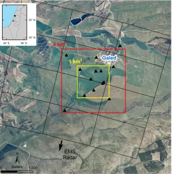
Fig. 1. Map of the study area including the 14 rain stations (triangles) around Kibbutz Galed. Each station is composed of two rain gauges. The black grid represents the radar mesh, with a spatial polar resolution of 1.4◦×1 km. Inset shows the general location of the network in Israel (star) and the location of the EMS weather radar (cross).

and nonconvective rainfall; (2) the number of rain gauges required to adequately measure rainfall in a radar subpixel scale; and (3) the decision as to which radar temporal reso-lution should be used for hydrological modeling due to the radar errors at the pixel scale. The paper is composed of six sections: Sect. 2 is dedicated to technical information regard-ing the rain gauge network’s installation and data quality control (QC). This section also contains information about the weather radar and rainfall estimations. The rainfall spa-tial correlation is described in Sect. 3. The uncertainty quan-tification for the mean areal rainfall representing the subpixel level is discussed in Sect. 4. The radar rainfall error variance and the radar evaluation are presented in Sect. 5. The con-clusions, discussion on the lessons learned, and near-future plans for the rain-gauge network are presented in Sect. 6.

2 Data

2.1 Galed dense rain-gauge network

Table 1. Intra-distances (m) of the rain stations.

1

1 0 2

2 1709 0 3

3 2672 1735 0 4

4 1457 620 1375 0 5

5 1395 1076 1277 456 0 6

6 1102 1052 1572 497 298 0 7

7 990 1193 1684 658 413 162 0 8

8 1699 1918 1444 1298 842 962 912 0 9

9 1920 1386 777 829 548 843 930 785 0 10

10 1620 1392 1111 778 354 598 645 557 336 0 11

11 1250 1448 1516 846 419 426 363 549 740 406 0 12

12 1303 1440 1461 831 392 438 395 525 685 350 57 0 13

13 686 1518 2057 1049 812 570 412 1019 1284 963 572 628 0 14

14 830 940 1938 634 708 434 450 1362 1253 1032 813 841 610 0

8 gauges deployed in a 4 km2 area of the Brue catchment (Moore et al., 2000).

The stations are distributed in a nonuniform design (Fig. 1), according to the terrain’s limitations (e.g. field crops, small streams, woods). The intra-distances of the rain sta-tions (see Table 1) vary between 57 and 2,672 m. Each station consists of two high-precision tipping-bucket rain gauges separated by about 1 m (as suggested by Ciach and Krajew-ski, 1999; Krajewski et al., 2003) to maintain better quality control and to acquire data on the zero-distance correlation of the rainfall. The tipping-bucket rain gauge was manufac-tured by YOUNG Company (model 52203). It has an orifice diameter of 18 cm with rainfall measurement resolution of 0.1 mm per tip and accuracy of 3 % up to 50 mm h−1. Each rain gauge is connected to a HOBO data logger (model UA-003-64). The maximum sampling frequency of the data log-ger is 1 Hz, with a memory of 64 K bytes (more than enough for 1 yr of measurements). This stands with the recommen-dations by Habib et al. (2001b) and Wang et al. (2008) to use a gauge bucket size of up to 0.254 mm with a temporal resolution of 1 s. The HOBO logger’s time accuracy is about 1 min per month. The loggers were synchronized each time the data were downloaded (approximately every three weeks) to minimize the potential problem of the loggers clocks’ drift. In addition, we used 1 min time intervals accumulated from the 1 s temporal resolution to reduce errors.

The study area has a Mediterranean climate; its rainy season lasts from October to May (mean annual rainfall is 550 mm), while June to September are typically dry and hot. In this study, we present the analysis of the first year record collected from 1 November 2011 to 1 May 2012. The ac-cumulated rainfall for this period, indicated by counting the number of tips in 1 min time intervals, is equal to 512 mm (averaged over the rain gauges) and is divided into 63 rain events. A rain event is defined as beginning when the first rain tip is detected in one of the rain gauges and ending when there is an intermission of more than 15 min in rainfall for

all gauges. Rain events with cumulative rainfall depth of less than 0.5 mm for all gauges were excluded. An inherent prob-lem with tipping-bucket-derived rain intensities is that only the time at which the bucket is completely filled is recorded and no information is available on the actual period of time it took to get filled. To overcome this problem, a backward linear interpolation to the previous recorded tip was applied, with two exceptions: (1) the time interval from the previous tip was larger than 15 min, or (2) this was the first tip in the rain event. Note that low rain intensities are more vulnerable to the above-mentioned problem.

To ensure reliability of the results, QC procedures were conducted. This is essential, as the data collected from the rain gauges may be corrupted due to partial clogging of the funnel by debris or small living creatures (for example, wasps or snails), or technical problems (such as a low battery) re-sulting in lack of measurements at a given time. Most of the errors were detected by comparing the rain intensity of rain gauge couples at each station and the rain event. In addition, the rain intensities of all of the gauges were compared for each rain event. All data which were considered to be cor-rupted were removed during the QC, ensuring a lack of intra-and inter-station measurement errors. After QC, rain inten-sity time series for time intervals between 1 min and daily timescales were computed for each rain gauge.

2.2 Radar data

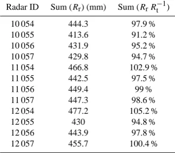
Table 2. Radar pixels afterZ–Rbias adjustment. Sum (Rr) repre-sents the accumulated rainfall for the studied period and Sum (Rr R_t−1) is the ratio between radar rainfall and rain gauge rainfall (av-eraged over the gauges) for the studied period.

Radar ID Sum (Rr) (mm) Sum (RrR−1t )

10 054 444.3 97.9 %

10 055 413.6 91.2 %

10 056 431.9 95.2 %

10 057 429.8 94.7 %

11 054 466.8 102.9 %

11 055 442.5 97.5 %

11 056 449.4 99 %

11 057 447.3 98.6 %

12 054 477.2 105.2 %

12 055 430 94.8 %

12 056 443.9 97.8 %

12 057 455.7 100.4 %

250 kW, a temporal resolution of about 3 min per volume scan, and a spatial polar resolution of 1.4◦×1 km in space (see grid in Fig. 1). Data from an elevation angle of 1◦(mean elevation of 1255 m above the network) were used for the analysis. No pixels with substantial ground clutter or beam blockage were detected in the analyzed region.

A total of 11 827 radar volume scans were analyzed in this study. The radar was shut down by the EMS for short pe-riods due to malfunctions and for regular maintenance, and thus 462 mm of rainfall were recorded by the radar out of the full 512 mm of rainfall recorded by the rain gauges. We chose 12 radar pixels over the network location and its sur-roundings for the analysis (Fig. 1) as the area of the gauge network is similar to that of 2–4 joint radar pixels (approxi-mately 4 km2).

Rainfall intensity data (R, mm h−1) were calculated from the weather radar reflectivity data (Z, mm6m−3) by a fixed Z–R power law relationship adjusted using the annual cu-mulative rainfall amount derived from the dense rain-gauge network. TheZ–R relationships were fixed toZ=126R1.5 for the radar pixels; a summarization of the adjustment is given in Table 2. Prior to this adjustment, the radar reflectiv-ity values were increased by 6 dB to compensate for system losses, as done by Morin and Gabella (2007). A lower thresh-old of 0.1 mm h−1for noise filtering and an upper threshold of 250 mm h−1to reduce unrealistically strong returns from hail particles were set.

In Fig. 2, scatter plots of synchronous radar (averaged data from the 12 pixels) and rain gauge observations are presented for three timescales: 3 min (the time interval between the radar volume scans), hourly and daily intervals. Ciach and Krajewski (1999) noted that this plot can give an idea of the large amount of variability in the measurements. Here we can see that for the shorter temporal resolution and for the lower rain intensity, the points scatter away from the perfect match

line of the radar-to-gauge amounts, possibly due to the prob-lem mentioned above with the unknown tipping-bucket fill time (see previous section).

3 Spatial correlation of gauge rainfall data

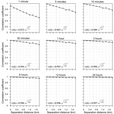
The spatial rainfall correlation is commonly investigated us-ing Pearson’s product–moment correlation (for examples, see Ciach and Krajewski, 2006; Mandapaka et al., 2010; Ped-ersen et al., 2010; Tokay and Ozturk, 2012; Villarini et al., 2008, and more). Correlograms for different timescales, from 1 min to daily, were computed using a lag distance of 200 m (Fig. 3). As expected, the spatial correlation decreased as the separation distance increased and as the timescale decreased. This trend was also shown by Krajewski et al. (2003) for several different experiments conducted worldwide, as well as by Ciach and Krajewski (2006) and Villarini et al. (2008). The correlation was parameterized using a three-parameter exponential function (see fit in Fig. 3), as suggested by Ge-bremichael and Krajewski (2004), Habib et al. (2001a) and Villarini et al. (2008), for the spatial correlation at separation distancehof the correlogram:

r(h)=c1·exp

− _h

c2 c3

, (1)

wherec1represents the nugget (zero-distance correlation),c2 is the correlation distance andc3is the shape factor.

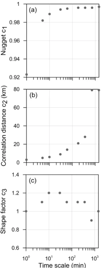
The time dependence of the parameters given in Eq. (1) are summarized in Fig. 4. The nugget has a value of about 0.92 on the 1 min scale, increasing to 0.98 for the 5 min scale and then continuing asymptotically toward 1 on the daily scale. The nugget represents the zero-distance correlation, thus it gives us information about the variability and mea-surement errors for each side-by-side rain gauge (i.e. each station); whenc1 is equal to 1 there is a perfect match be-tween the side-by-side gauges. The values obtained in this study were much higher than those reported by Villarini et al. (2008) of c1=0.5 on the 1 min timescale; they are on a scale similar to the values given by Krajewski et al. (2003) ofc1=0.95–0.97 (different locations worldwide) on timescales of 15 min or longer. Tokay and Ozturk (2012) re-ported values ofc1=0.97 on a 5 min timescale.

Fig. 2. Scatter plots of synchronous radar and rain gauge observations for 3 min (radar data are transected along the lower 0.1 mm h−1rainfall intensity threshold), hourly and daily intervals. The radar rainfall data represent the averaged rainfall derived from the 12 radar pixels. Dashed line represents a perfect fit between gauge and radar rainfall.

Fig. 4. Time-scale dependence of the nugget (a), correlation dis-tance (b) and shape factor (c) used in the three-parameter exponen-tial function.

In this study, the shape parameter (c3) was approximately 1 (a pure exponential function), slightly changing from 0.9 to 1.2 with no obvious trend. The shape parameter function estimated in this study was different from those obtained by Ciach and Krajewski (2006), Tokay and Ozturk (2012), and Villarini et al. (2008), where an increase in the shape param-eter was detected with an increase in the timescale (between 1.1 and 1.6, 0.37 and 0.92 and 0.4 and 1, respectively). As Villarini et al. (2008) mentioned, differences are expected be-tween experimental studies due to differences in the range of inter-gauge distances, sample size and precipitation type.

4 Spatial rain gauge uncertainty

4.1 Variance reduction factor

The rainfall variance was estimated by the well-known vari-ance reduction factor (VRF), which has been used by Kra-jewski et al. (2000) and Villarini et al. (2008) to quantify the uncertainty results from averaging a number of rain gauges. The VRF methodology was introduced by Rodr´ıguez-Iturbe and Mej´ıa (1974) and Bras and Rodr´ıguez-Iturbe (1976). Morrissey et al. (1995) proposed a numerical method which considered the number of rain gauges, their spatial distribu-tion, and the correlation between them. In this paper, we pro-vide only a brief discussion of the VRF methodology; for further details, the reader is referred to the above-mentioned papers.

LetRs be the point rainfall of a single rain station (two side-by-side gauges per station), Rs be the averaged-areal rainfall derived from the rain stations, and letRtbe the true areal rainfall. The mean square error of the true rainfall to the averaged-areal rainfall can be expressed as:

E[(Rt−Rs)2] =σR2s·VRF, (2)

whereσ_R2

sis the variance of the point rainfall and the VRF is

computed by

VRF= 1 n2·

N X

i=1 N X

j=1

ρ(di,j)·δ(i)·δ(j )− 2 N·n

· N X

i=1 N X

j=1

ρ(di,j)·δ(i)+ 1 N +

2 N2·

N−1 X

i=1 N X

j=i+1

ρ(di,j), (3)

wherenis the number of rainfall measuring stations,Nis the number of boxes dividing the domain,ρ(di,j)is the correla-tion coefficient derived from Eq. (1) for the distance between boxesi andj, andδ is a Boolean value with a value of 1 when boxicontains a measuring station (each box can con-tain only one measuring station) and a value of 0 otherwise.

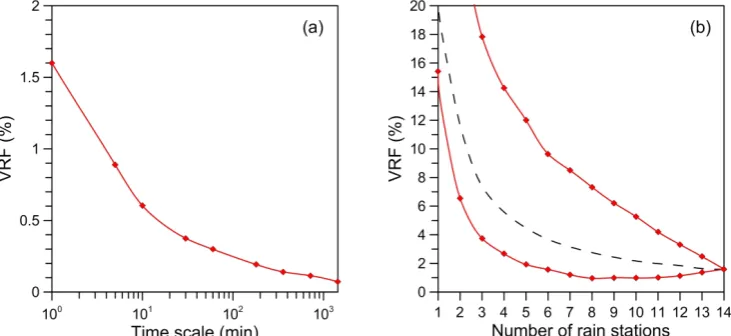
The domain area was defined with dimensions of 2.1×2.1 km in order to capture all of the rain stations (n= 14) participating in this study (Fig. 1; see the 4 km2 box for comparison). The grid was composed of 441 boxes (N), each with a size of 100×100 m. The results are plotted in Fig. 5a. The VRF was 1.6 % for a timescale of 1 min and it decreased with increasing time accumulated to 0.07 % for the daily timescale. These results are similar to those presented by Villarini et al. (2008) for a 4 km2domain, where the VRF decreased from approximately 2.7 % for a timescale of 1 min to near zero for the daily timescale. The VRF is very close to zero, meaning that the left side of Eq. (2) is also close to zero; thus for any given timescale, the true rainfall will be well represented by the averaged-areal rainfall.

Fig. 5. Variance reduction factor (VRF) as a function of (a) timescale and (b) number of rain stations in the study area for the 1 min timescale (maximum, minimum and median).

The VRF was computed from one station to 14 stations where all possible combinations were calculated. As the re-sults for the different timescales are similar, only the rere-sults for the 1 min timescale are plotted in Fig. 5b and discussed here. Examining the minimum VRF values suggested that setting up three rain stations in a specific configuration within a radar pixel domain is sufficient to represent the rainfall within the radar pixel, assuming that the VRF threshold of 5 % is satisfied. VRF values lower than 2 % will require at least five rain stations in the domain. The lowest VRF was found for the setting of 10 rain stations (0.99 %) in the do-main. The VRF increases with the addition of more than 10 rain stations as the distances between the rain stations de-crease, resulting in an increase of the first term in Eq. (3). 4.2 Convective rainfall

The contribution of convective rainfall to the total precipi-tation over the study area cannot be overlooked. To check whether there are differences in the spatial correlation of the convective versus nonconvective rainfall, we divided the rainfall series at the 5 min timescale as follows: if at least one of the rain gauges recorded rain intensity exceeding 10 mm h−1, this 5 min interval was marked as convective (it was summed up to 242 mm – about 47 % of the total measured rainfall); if all rain gauges recorded rain intensity lower than 10 mm h−1, it was marked as nonconvective. This threshold was used by Peleg and Morin (2012) to distinguish the convective rain cells from the total precipitation in the same area.

The spatial correlation for the convective and nonconvec-tive rainfall for the 5 min timescale was calculated using the methodology explained in Sect. 3, and is presented in Fig. 6a. The nugget of the convective precipitation is 0.97, while the nugget of the nonconvective rainfall is 0.95. The convective spatial correlation decreases rapidly to 0.4 at a separation

dis-tance of 1.8 km, while the nonconvective spatial correlation decreases more moderately to 0.7 at the same distance. The nonconvective spatial correlation decays in a manner simi-lar to the 5 min correlation decay of the combined convective and nonconvective rainfall presented in Fig. 3. The fast de-cay of the convective rainfall spatial correlation implies that the areal rainfall variance is high. The standard deviation of the convective rainfall, normalized by its mean, was plotted against the fraction of rain gauges exceeding the threshold of 10 mm h−1 (Fig. 6b). The normalized standard deviation (NSTD) of the convective rainfall is about 0.4. The maxi-mum NSTD is higher for fewer rain gauges that detect rain intensity exceeding the threshold.

5 Radar estimation error

5.1 Error separation method

Ciach and Krajewski (1999) proposed the error separation method (ESM) which separates the radar–rain gauge error in two: the radar–true area-averaged rainfall error and the rain gauge sampling error. Below is a short description of the method; for further information the reader is referred to Ciach and Krajewski (1999) and to an additional example by Krajewski et al. (2000).

Let Rr be the rainfall estimated from the radar, Rg the rainfall as measured by the rain gauge andRtthe true area-averaged rainfall. The normalized root mean square error of the radar-estimated rainfall versus the rain gauges is found by

NRMSE(Rr−Rg)= r

PN

i=1(Rr(i)−Rg(i))2

N

Rg

Fig. 6. (a) Correlogram presenting the convective (red plus symbol) and nonconvective (blue dots) spatial rainfall coefficient and its fit (dashed lines) using the three-parameter exponential functions. (b) Convective rain intensity normalized standard deviation. The analysis was performed for the 5 min rain intensity data.

whereN is the sample size andRg is the averaged rainfall measured by the gauges. The normalized rain gauge sam-pling error can be determined (based on Eq. (18) in Ciach and Krajewski, 1999) by

NRMSE(Rg−Rt)= p

var(Rg)·(1−c1)

Rg , (5)

wherec1is the nugget. The radar–true area-averaged rainfall error can be then solved by

var{Rr−Rt} =varRr−Rg −varRg−Rt , (6) where var

Rr−Rg and varRg−Rr are derived from Eqs. (4) and (5), respectively. For the above computation, we assume that there is no bias between the rainfall measured by the rain gauges and the rainfall measured by the weather radar, as each radar pixel is adjusted separately for the data derived from the gauges.

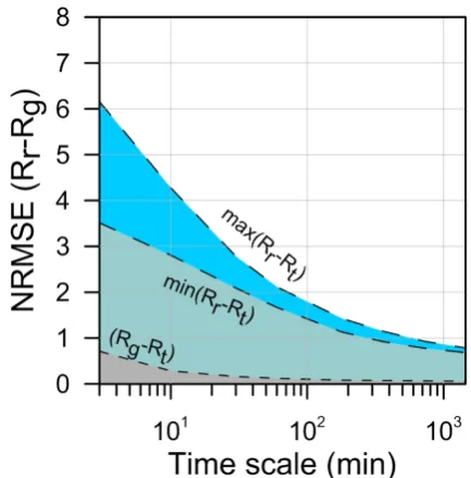
The results of the ESM for the different timescales are pre-sented in Fig. 7 for the relative magnitude of each of the method components. The normalized radar–true rainfall er-ror is presented for the maximum and minimum values ob-tained from the 12 radar pixels tested (i.e. maximum and minimum values represent one pixel each and the other 10 pixel values are found in the range between). The radar rain-gauge error declines from a maximum 615 % error (mini-mum of 351 %) for a timescale of 3 min to a maxi(mini-mum 78 % error (minimum 68 %) for the daily timescale. The error de-rived from the rain gauge sampling error is reduced from 71 % for a timescale of 3 min to 5 % for a daily timescale. The gauge sampling error contributes only a relatively small part of the overall error: it changes from 20 % (minimum contribution of 11.5 %) for the 3 min timescale to 8 % (mini-mum of 7 %) for the daily timescale.

Fig. 7. Errors of radar (Rr) vs. gauge (Rg) rainfall for different timescales. The normalized root mean square errors of radar rain-fall (Rr) vs. true rainrain-fall (Rt) were analyzed independently for 12 radar pixels. The maximum and minimum are presented by the blue sections. Gray section represents the spatial sampling error derived from the rain gauge (Rg) vs. true areal rainfall (Rt).

5.2 Radar rainfall evaluation

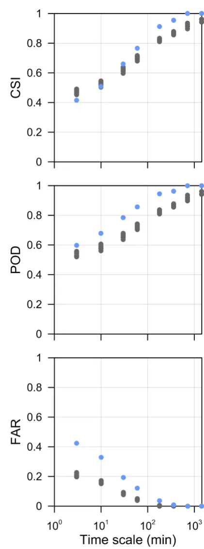
2009). These quality parameters are defined as

CSI= H

H+F+M (7)

FAR= F

H+F (8)

POD= H

H+M, (9)

whereHis the number of hits – both radar and gauged areal average rainfall indicate rain; M means number of misses – rainfall was only recorded by rain gauges;F means false alarms – rainfall was only recorded by radar. A zero threshold was used to mark the occurrence of rain. This means that the lower threshold for the radar was defined as 0.1 mm h−1(see Sect. 2.2), while the averaged gauged rainfall was indicative for rain as at least one rain gauge recorded rain.

The evaluation was conducted for different timescales for each of the radar pixels and for the radar pixel average, and the results are presented in Fig. 8. All quality parameters im-proved as the timescale increased, in a manner similar to the ESM results discussed in the previous section. The CSI for the averaged radar pixel changed from 0.41 for the 3 min timescale to 1 for the daily timescale and its POD increased from 0.6 to 1 for the same timescales. The FAR decreased from 0.42 for the 3 min timescale to zero for the 3 h timescale and on. These results are affected by the threshold set to de-fine a rain occurrence, where higher threshold changes the CSI, POD and FAR results.

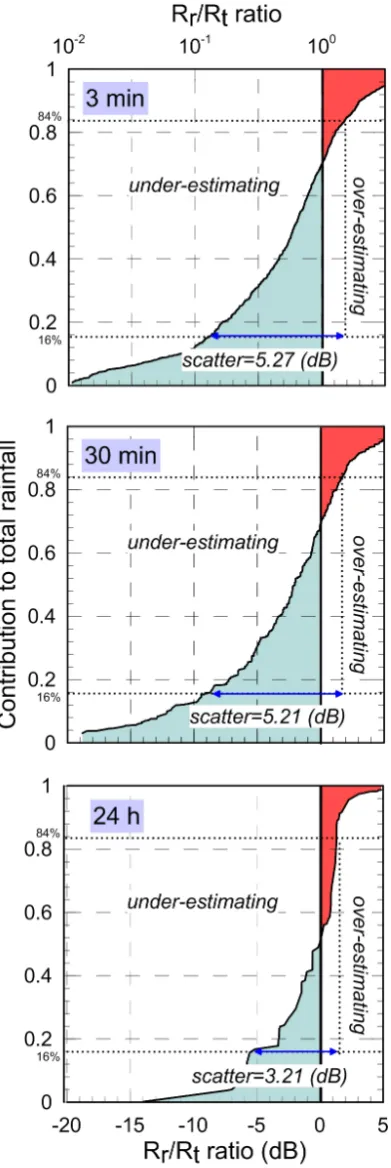
The ratio of averaged radar rainfall to true areal rainfall was calculated for 3 min, 30 min and daily timescales. Here, we assumed that the true rainfall is well represented by the areal-averaged gauge-derived rainfall. The cumulative dis-tribution (weighted by condis-tribution to total rain amount) of the radar-to-true rainfall ratio (in dB) is presented in Fig. 9, following Germann et al. (2006). For the 3 min timescale, the radar underestimated about 70 % of the rainfall, with the radar-to-true rainfall ratio reaching up to −22 dB. For the daily timescale, the radar estimations improved, with the inflection point between the under- and overestimation found around the 50 % rainfall contribution and the radar-to-true rainfall ratio being as low as−14 dB. The improve-ment of the radar estimation for the true rainfall with in-creasing timescale was also expressed by the scatter param-eter, defined as half the distance between the 16th and 84th percentiles of the error distribution (Germann et al., 2006). The scatter decreased from 5.27 dB for the 3 min timescale to 3.21 dB for the daily timescale.

6 Conclusions

Subpixel rain distribution was investigated using a high-density network of rain gauges within a 4 km2 area as a part of continuous efforts to better understand the uncertain-ties and errors of rainfall estimation at this scale. This is

Fig. 9. Cumulative distribution (weighted by contribution to total rain amount) of the radar-to-true rainfall ratio (Rr/Rt, in dB) (see Germann et al., 2006) for different timescales.

of particular importance when using remote sensing rainfall data (from ground weather radar or from satellite) for hydro-logical applications. In this study, we used the network of 27 tipping-bucket rain gauges located in northern Israel to eval-uate the Shacham weather radar’s performance and to learn about small-scale rainfall variability. From the first year of observation three lessons were learned:

– First, we examined the spatial correlation of gauge rainfall data as has been done before for different lo-cations worldwide. We found that the nugget (zero-distance correlation) between rain gauges is high (0.92 for the 1 min timescale) and it increases with increasing timescale. Moreover, spatial rainfall correlations for all separation distances generally increase with timescale. The more important finding was that there is a differ-ence in spatial correlations between convective and non-convective rainfall, where the non-convective rainfall corre-lation decreases much faster with distance than the non-convective. Convective rainfall correlations have long been a subject for study (for example, see papers by Sharon, 1974; Osborn et al., 1979) but, to the best of our knowledge, this is the first time that this examina-tion has been performed at the radar pixel scale. The fast decay of convective rainfall correlation within a radar pixel may imply that the radar errors for high rainfall intensity are even larger than thought. Further investi-gation is needed to understand the spatial and temporal differences between the different types of rainfall and its effects on radar data.

while our results indicate that to remove uncertainties related to subpixel rainfall distribution three rain gauges per pixel are better, at least for a similar climate. Obvi-ously, this will increase the cost of such a network; how-ever, it will also assure meaningful validation results. – Lastly, we debate the question of which radar temporal

resolution should be used for hydrological applications. A possible answer to this question is to fit the required temporal resolution to the basin hydrological response that depends on catchment size, land use and other prop-erties (Morin et al., 2001). Berne et al. (2004) sug-gested a temporal scale of 3–5 min for urban catchments of the order of 1–10 km2, while Atencia et al. (2011) suggested a temporal scale of 12–15 min for basins of the order of 100–1000 km2_{. Another aspect to consider} is radar errors for the pixel scale and its change with time (Fig. 7). It was found that the radar–rain gauge error decreases from 477 % for the 3 min timescale to 345 % for the 10 min scale and down to 72 % for the daily timescale (all are areal mean values). This error is mainly the result of radar estimation errors, as the gauge sampling error contributes only 8–20 % to the total er-ror, depending on the timescale. The improvement in radar rainfall estimations with increasing timescale is reflected by the increase of the CSI and POD parame-ters with timescale and the simultaneous decrease of the FAR parameter. In addition, the radar-to-true rainfall ra-tio, expressed by the scatter parameter, decreases with increasing timescale from 5.27 dB for the 3 min scale to 3.21 dB for the daily scale. Based on these results, we recommend utilizing the radar rainfall data at scales of at least 10 min, thus benefiting from the large reduction in error from 3 min timescale to the 10 min scale. We intend to continue collecting rainfall measurements with this network of rain gauges in the years to come. In De-cember 2012, a disdrometer was installed at this site to mea-sure rain drop size distribution (e.g., Jaffrain et al., 2011). We are looking for new and better ways to continue devel-oping this network for future use with other weather radar or satellite observations.

Acknowledgements. The authors thank Kibbutz Galed for their

valuable assistance and cooperation and also to Camille Vainstein for her editorial work. The research was supported by the Israeli Ministry of Environmental Protection and THE ISRAEL SCIENCE FOUNDATION – The Recanati and IDB Group Foundation (grant No. 332/11). We thank the two reviewers (Hidde Leijnse and the second anonymous reviewer) and the editor for their significant contribution to the quality of the paper.

Edited by: A. Langousis

References

Amitai, E., Unkrich, C. L., Goodrich, D. C., Habib, E., and Thill, B.: Assessing satellite-based rainfall estimates in semi-arid watersheds using the USDA-ARS walnut gulch gauge network and TRMM PR, J. Hydrometeorol., 13, 1579–1588, doi:10.1175/jhm-d-12-016.1, 2012.

Arnaud, P., Lavabre, J., Fouchier, C., Diss, S., and Javelle, P.: Sensitivity of hydrological models to uncertainty in rain-fall input, Hydrol. Sci. J.-J. Sci. Hydrol., 56, 397–410, doi:10.1080/02626667.2011.563742, 2011.

Atencia, A., Mediero, L., Llasat, M. C., and Garrote, L.: Effect of radar rainfall time resolution on the predictive capability of a dis-tributed hydrologic model, Hydrol. Earth Syst. Sci., 15, 3809– 3827, doi:10.5194/hess-15-3809-2011, 2011.

Bahat, Y., Grodek, T., Lekach, J., and Morin, E.: Rainfall-runoff modeling in a small hyper-arid catchment, J. Hydrol., 373, 204– 217, doi:10.1016/j.jhydrol.2009.04.026, 2009.

Berne, A. and Krajewski, W. F.: Radar for hydrology: Unfulfilled promise or unrecognized potential?, Adv. Water Resour., 51, 357–366, doi:10.1016/j.advwatres.2012.05.005, 2013.

Berne, A., Delrieu, G., Creutin, J. D., and Obled, C.: Tem-poral and spatial resolution of rainfall measurements re-quired for urban hydrology, J. Hydrol., 299, 166–179, doi:10.1016/j.jhydrol.2004.08.002, 2004.

Bras, R. L. and Rodr´ıguez-Iturbe, I.: Evaluation of mean square error involved in approximating the areal average of a rainfall event by a discrete summation, Water Resour. Res., 12, 181–184, doi:10.1029/WR012i002p00181, 1976.

Ciach, G. J.: Local random errors in tipping-bucket rain gauge measurements, J. Atmos. Ocean. Technol., 20, 752–759, doi:10.1175/1520-0426(2003)20<752:lreitb>2.0.co;2, 2003. Ciach, G. J. and Krajewski, W. F.: On the estimation of radar

rainfall error variance, Adv. Water Resour., 22, 585–595, doi:10.1016/s0309-1708(98)00043-8, 1999.

Ciach, G. J. and Krajewski, W. F.: Analysis and model-ing of spatial correlation structure in small-scale rainfall in Central Oklahoma, Adv. Water Resour., 29, 1450–1463, doi:10.1016/j.advwatres.2005.11.003, 2006.

Dixon, M. and Wiener, G.: TITAN – thunderstorm identification, tracking, analysis, and nowcasting – a radar-based methodol-ogy, J. Atmos. Ocean. Technol., 10, 785–797, doi:10.1175/1520-0426(1993)010<0785:ttitaa>2.0.co;2, 1993.

Faures, J. M., Goodrich, D. C., Woolhiser, D. A., and Sorooshian, S.: Impact of small-scale spatial rainfall variability on runoff modeling, J. Hydrol., 173, 309–326, doi:10.1016/0022-1694(95)02704-s, 1995.

Fiener, P. and Auerswald, K.: Spatial variability of rainfall on a sub-kilometre scale, Earth Surf. Proc. Land., 34, 848–859, doi:10.1002/esp.1779, 2009.

Gebremichael, M. and Krajewski, W. F.: Assessment of the statistical characterization of small-scale rainfall variabil-ity from radar: Analysis of TRMM ground validation datasets, J. Appl. Meteorol., 43, 1180–1199, doi:10.1175/1520-0450(2004)043<1180:aotsco>2.0.co;2, 2004.

Germann, U., Galli, G., Boscacci, M., and Bolliger, M.: Radar pre-cipitation measurement in a mountainous region, Q. J. Roy. Me-teor. Soc., 132, 1669–1692, doi:10.1256/qj.05.190, 2006. Habib, E., Krajewski, W. F., and Ciach, G. J.: Estimation of

doi:10.1175/1525-7541(2001)002<0621:eoric>2.0.co;2, 2001a.

Habib, E., Krajewski, W. F., and Kruger, A.: Sampling errors of tipping-bucket rain gauge measurements, J. Hydrol. Eng., 6, 159–166, doi:10.1061/(asce)1084-0699(2001)6:2(159), 2001b. Jaffrain, J., Studzinski, A., and Berne, A.: A network of

dis-drometers to quantify the small-scale variability of the rain-drop size distribution, Water Resour. Res., 47, W00h06, doi:10.1029/2010wr009872, 2011.

Jensen, N. E. and Pedersen, L.: Spatial variability of rainfall: Vari-ations within a single radar pixel, Atmos. Res., 77, 269–277, doi:10.1016/j.atmosres.2004.10.029, 2005.

Karklinsky, M. and Morin, E.: Spatial characteristics of radar-derived convective rain cells over southern Israel, Meteorol. Z., 15, 513–520, doi:10.1127/0941-2948/2006/0153, 2006. Krajewski, W. F. and Smith, J. A.: Radar hydrology: rainfall

esti-mation, Adv. Water Resour., 25, 1387–1394, doi:10.1016/s0309-1708(02)00062-3, 2002.

Krajewski, W. F., Kruger, A., and Nespor, V.: Experimental and nu-merical studies of small-scale rainfall measurements and vari-ability, Water Sci. Technol., 37, 131–138, doi:10.1016/s0273-1223(98)00325-4, 1998.

Krajewski, W. F., Ciach, G. J., McCollum, J. R., and Ba-cotiu, C.: Initial validation of the global precipitation cli-matology project monthly rainfall over the United States, J. Appl. Meteorol., 39, 1071–1086, doi:10.1175/1520-0450(2000)039<1071:ivotgp>2.0.co;2, 2000.

Krajewski, W. F., Ciach, G. J., and Habib, E.: An analysis of small-scale rainfall variability in different climatic regimes, Hydrol. Sci. J., 48, 151–162, doi:10.1623/hysj.48.2.151.44694, 2003. Krajewski, W. F., Villarini, G., and Smith, J. A.: Radar-rainfall

un-certainties – where are we after thirty years of effort?, B. Am. Meteorol. Soc., 91, 87–94, doi:10.1175/2009bams2747.1, 2010. Kyznarova, H. and Novak, P.: CELLTRACK – Convec-tive cell tracking algorithm and its use for deriving life cycle characteristics, Atmos. Res., 93, 317–327, doi:10.1016/j.atmosres.2008.09.019, 2009.

Mandapaka, P. V., Villarini, G., Seo, B. C., and Krajewski, W. F.: Effect of radar-rainfall uncertainties on the spatial characteriza-tion of rainfall events, J. Geophys. Res.-Atmos., 115, D17110, doi:10.1029/2009jd013366, 2010.

Moore, R. J., Jones, D. A., Cox, D. R., and Isham, V. S.: Design of the HYREX raingauge network, Hydrol. Earth Syst. Sci., 4, 521–530, doi:10.5194/hess-4-521-2000, 2000.

Morin, E. and Gabella, M.: Radar-based quantitative precipitation estimation over Mediterranean and dry climate regimes, J. Geo-phys. Res.-Atmos., 112, D20108, doi:10.1029/2006jd008206, 2007.

Morin, E., Enzel, Y., Shamir, U., and Garti, R.: The character-istic time scale for basin hydrological response using radar data, J. Hydrol., 252, 85–99, doi:10.1016/s0022-1694(01)00451-6, 2001.

Morin, E., Goodrich, D. C., Maddox, R. A., Gao, X. G., Gupta, H. V., and Sorooshian, S.: Spatial patterns in thun-derstorm rainfall events and their coupling with watershed hydrological response, Adv. Water Resour., 29, 843–860, doi:10.1016/j.advwatres.2005.07.014, 2006.

Morin, E., Jacoby, Y., Navon, S., and Bet-Halachmi, E.: To-wards flash-flood prediction in the dry Dead Sea region utilizing

radar rainfall information, Adv. Water Resour., 32, 1066–1076, doi:10.1016/j.advwatres.2008.11.011, 2009.

Morrissey, M. L., Maliekal, J. A., Greene, J. S., and Wang, J. M.: THe uncertainty of simple spatial averages using rain-gauge networks, Water Resour. Res., 31, 2011–2017, doi:10.1029/95wr01232, 1995.

Nikolopoulos, E. I., Anagnostou, E. N., Hossain, F., Gebremichael, M., and Borga, M.: Understanding the scale relationships of uncertainty propagation of satellite rainfall through a dis-tributed hydrologic model, J. Hydrometeorol., 11, 520–532, doi:10.1175/2009jhm1169.1, 2010.

Osborn, H. B., Renard, K. G., and Simanton, J. R.: Dense networks to measure convective rainfall in the southwest-ern United States, Water Resour. Res., 15, 1701–1711, doi:10.1029/WR015i006p01701, 1979.

Pedersen, L., Jensen, N. E., Christensen, L. E., and Madsen, H.: Quantification of the spatial variability of rainfall based on a dense network of rain gauges, Atmos. Res., 95, 441–454, doi:10.1016/j.atmosres.2009.11.007, 2010.

Peleg, N. and Morin, E.: Convective rain cells: Radar-derived spatiotemporal characteristics and synoptic patterns over the eastern Mediterranean, J. Geophys. Res., 117, D15116, doi:10.1029/2011jd017353, 2012.

Rodr´ıguez-Iturbe, I. and Mej´ıa, J. M.: The design of rainfall net-works in time and space, Water Resour. Res., 10, 713–728, doi:10.1029/WR010i004p00713, 1974.

Rozalis, S., Morin, E., Yair, Y., and Price, C.: Flash flood prediction using an uncalibrated hydrological model and radar rainfall data in a Mediterranean watershed under changing hydrological conditions, J. Hydrol., 394, 245–255, doi:10.1016/j.jhydrol.2010.03.021, 2010.

Seo, B. C. and Krajewski, W. F.: Investigation of the scale-dependent variability of radar-rainfall and rain gauge error covariance, Adv. Water Resour., 34, 152–163, doi:10.1016/j.advwatres.2010.10.006, 2011.

Sharon, D.: The spatial pattern of convective rainfall in Sukuma-land, Tanzani – A statistical analysis, Arch. Met. Geoph. Biokl. B., 22, 201–218, doi:10.1007/bf02243468, 1974.

Singh, V. P.: Effect of spatial and temporal variability in rain-fall and watershed characteristics on stream flow hydro-graph, Hydrol. Process., 11, 1649–1669, doi:10.1002/(sici)1099-1085(19971015)11:12<1649::aid-hyp495>3.0.co;2-1, 1997. Tapiador, F. J., Checa, R., and de Castro, M.: An experiment to

measure the spatial variability of rain drop size distribution us-ing sixteen laser disdrometers, Geophys. Res. Lett., 37, L16803, doi:10.1029/2010gl044120, 2010.

Tokay, A. and Ozturk, K.: An Experimental Study of the Small-Scale Variability of Rainfall, J. Hydrometeorol., 13, 351–365, doi:10.1175/jhm-d-11-014.1, 2012.

Tokay, A. and Bashor, P. G.: An Experimental Study of Small-Scale Variability of Raindrop Size Distribution, J. Appl. Mete-orol. Clim., 49, 2348–2365, doi:10.1175/2010jamc2269.1, 2010. Villarini, G., Mandapaka, P. V., Krajewski, W. F., and Moore, R. J.: Rainfall and sampling uncertainties: A rain gauge perspective, J. Geophys. Res.-Atmos., 113, D11102, doi:10.1029/2007jd009214, 2008.

Wood, S. J., Jones, D. A., and Moore, R. J.: Accuracy of rainfall measurement for scales of hydrological interest, Hydrol. Earth Syst. Sci., 4, 531–543, doi:10.5194/hess-4-531-2000, 2000. Yakir, H. and Morin, E.: Hydrologic response of a semi-arid

wa-tershed to spatial and temporal characteristics of convective rain cells, Hydrol. Earth Syst. Sci., 15, 393–404, doi:10.5194/hess-15-393-2011, 2011.