Complex Nonlinear System Modelling and Parameters Identification by Deep Neural Networks

2019 International Conference on Artificial Intelligence, Control and Automation Engineering (AICAE 2019) ISBN: 978-1-60595-643-5

Complex Nonlinear System Modelling and Parameters Identification by

Deep Neural Networks

Hai-long LIN

, Gao-yong LUO

, Hai-tao CAO

,

Xiao-hui FANG

and Fa-sheng ZHOU

1_{School of Physics and Electronics Engineering, Guangzhou University, Guangzhou, China}

2_{Department of Information Engineering, Padova University, Padova, Italy}

*Corresponding author

Keywords: Complex nonlinear system, Deep neural networks, Parameters identification, Machine learning.

Abstract. As most systems are inherently nonlinear in nature, many efforts have been made to improve the understanding of complicated nonlinear models. However, current research has indicated that it is still a challenge to accurately model and identify nonlinear systems by conventional methods such as machine learning. This paper investigates a complex nonlinear system with three parameters identification by training a Deep Neural Network (DNN) to model the system based on Fourier series theory. The DNN with 10 layers is constructed such that it can model any nonlinear system, and the parameters identification is performed by the trained neural networks. The proposed method has been evaluated by applying to a nonlinear system for multiple parameters measurement by interferometric fiber sensors. Experimental results demonstrate that the DNN can accurately model the nonlinear system and identify the corresponding parameters, leading to a solution to complex nonlinear system approximation with minimized error.

Introduction

paper investigates a complex nonlinear system with three parameters identification by training a deep neural network to model the system based on Fourier series theory.

Nonlinear System Modelling and Identification

Deep Neural Networks Structure

With the improvement of computing capacity nowadays, AI technology has been widely used in many engineering applications. In particular, DNN theory has already been proposed to analyze nonlinear system. The deep structure of DNN strengthens its fitting capacity for complex nonlinear systems [13, 14]. The training process of DNN can be divided into forward-propagation and back-propagation [15]. Forward-propagation (FP)process can be written as

𝑦̃𝑙 _{= 𝑓}𝑙_(𝑧𝑙_{) = 𝑓}𝑙_(𝑊𝑙_𝑦̃𝑙−1_{+ 𝑏}𝑙_{) (1)}

where 𝑙 represents the index of layer, 𝑓𝑙(∙) is the activation function of layer 𝑙. The strong fitting capacity of DNN mainly comes from the activation functions used. 𝑊𝑙 and 𝑏𝑙 are the weights and bias of layer 𝑙, respectively. 𝑦̃ is the layer output data. Often for nonlinear tasks, there isn’t activation function in output layer. So the loss function can be written as

𝐽(𝑊, 𝑏, 𝑥, 𝑦) =_2𝑀1 ∑𝑀𝑖=1(𝑦̃𝑖− 𝑦𝑖)2 (2)

where 𝑀 is the length of 1D signal, 𝑦 is the desired output. Back-propagation (BP) algorithm [16] can then be expressed as

{

𝛿𝑊𝑙 = 𝜕𝐽(𝑊,𝑏,𝑥,𝑦)_𝜕𝑊𝑙 =

𝜕𝐽(𝑊,𝑏,𝑥,𝑦) 𝜕𝑧𝑙

𝜕𝑧𝑙

𝜕𝑊𝑙

𝛿_𝑏𝑙 ₌ 𝜕𝐽(𝑊,𝑏,𝑥,𝑦)

𝜕𝑏𝑙 =

𝜕𝐽(𝑊,𝑏,𝑥,𝑦) 𝜕𝑧𝑙

𝜕𝑧𝑙 𝜕𝑏𝑙

𝑊𝑛𝑒𝑤𝑙 = 𝑊𝑙− 𝛼𝛿𝑊𝑙 𝑏_𝑛𝑒𝑤𝑙 _{= 𝑏}𝑙_{− 𝛼𝛿}

𝑏𝑙

(3)

where 𝛼 represents learning rate, 𝑊_𝑛𝑒𝑤𝑙 and 𝑏_𝑛𝑒𝑤𝑙 are the updated weights and biases, respectively.

Nonlinear System Model of Interferometric Fiber Sensors (IFS)

IFS investigate two or more laser beams which exist optical path difference (OPD) while the wavelengths are identical. IFS have high sensitivity and resolution because the interference laser wavelength is ultrashort. Current research has shown that it can be used to measure multiple parameters of pressure and other applications [17]. The signal obtained from IFS can be written as

𝑦 = ∑ 𝐴_𝑖cos (𝑎𝑖

𝜆𝑘)

𝑁

𝑖=1 + 𝜂0+ 𝜂𝐷𝐶 (4)

where 𝜂₀ is random noise and 𝜂_𝐷𝐶 is DC component, 𝜆_𝑘 represents the uniform wavelength and is the input of output signal y, 𝐴𝑖 is signal amplitude and 𝑎𝑖 is optical path difference (OPD). 𝐴𝑖 and 𝑎𝑖 are

the model parameters which need to be estimated. 𝑁 represents the number of OPD. The relationship between input and output is nonlinear. After removing noise 𝜂₀ and 𝜂_𝐷𝐶, we can rewrite equation (4) as

𝑦 = ∑𝑁𝑖=1𝐴𝑖cos(𝑎𝑖𝑓𝑖𝑡𝑘) (5)

by Fourier Transform. This estimation also exists bias because the signal is non-uniform [19]. In next section, we propose a new method to accurately model and identify such a complex nonlinear system.

Proposed Method

Based on Fourier series theory, we propose a new method for analyzing IFS nonlinear system. After removing noise 𝜂0 and 𝜂𝐷𝐶, Fast Fourier Transform (FFT) can be applied on signal y. Among the

known 𝜆_𝑘, we found the minimum wavelength 𝜆_𝑚𝑖𝑛 and obtained the maximum frequency component 𝑓_𝑚𝑎𝑥 with well-known equation 𝑓_𝑚𝑎𝑥 = 𝐶 𝜆⁄ _𝑚𝑖𝑛. 𝐶 = 3 × 108m/s is the light speed. Then we assumed sampling frequency 𝑓_𝑠 = 2𝑓_𝑚𝑎𝑥. The major frequency components 𝑓₁… 𝑓_𝑁 could be estimated from the spectrum amplitudes by frequency analysis, so that the model parameters 𝑁 can be accurately identified.

Estimating the Values 𝑨_𝒊, 𝒇_𝒊 and 𝜽_𝒊

From equation (5), we know that signal 𝑦 is periodic. According to Fourier series theory, any periodic signal can be approximated with infinite sum of cosines and sines as:

𝑦 ≈ 𝑦̂ = 𝑎₀+ ∑ [𝐴_{𝑖 𝑖}cos(2𝜋𝑓_𝑖𝑡) + 𝐵_𝑖sin (2𝜋𝑓_𝑖𝑡)] (6) If the equation is couple function,the Fourier function can be wiritten as [20]

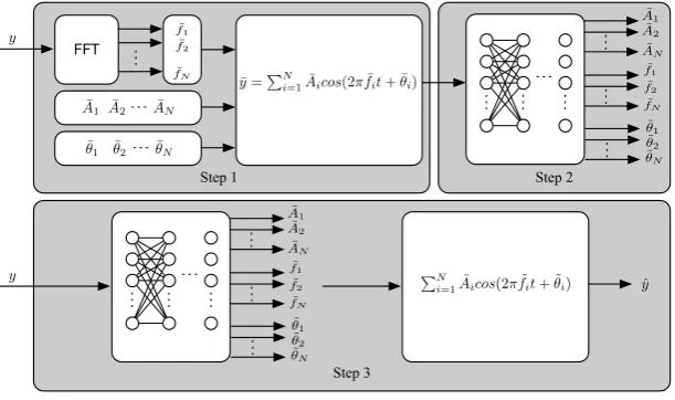
𝑦 ≈ 𝑦̂ = ∑ 𝐴_{𝑖 𝑖}cos(2𝜋𝑓_𝑖𝑡 + 𝜃_𝑖) (7) where 𝜃_𝑖 is initial phase. The amplitude values 𝐴_𝑖, initial phase values 𝜃_𝑖 and the frequency values 𝑓_𝑖 of cosine terms in equation (7) can be estimated by training a 10 layers DNN recursively. The loss function used is given in equation (2). The training process is to find a signal 𝑦̂ which is reconstructed by equation (7), in order to reach 𝑦 ≈ 𝑦̂. The proposed method is illustrated in figure 1.

Figure 1. The training process of the proposed method.

Before recursively training the built DNN model, a pre-training precedure (Step 1) has been set to initialize the weights of DNN. The output signal 𝑦̅ can then be taken as the first training data in Step 2. The output of DNN model is expected to approximate the pre-defined paramters as in Step 1, i.e.,

𝐴̅_𝑖, 𝑓̅_𝑖 and 𝜃̅_𝑖, 𝑖 = 1,2, … , 𝑁. In Step 3, the measured and denoised signal 𝑦 is fed into the pre-trained DNN model for recursively training the DNN (Step 2 and Step 3) until the reconstructed signal 𝑦̂ closely approximates the signal 𝑦 as described in equation (2). When the training process converges, the output of DNN in Step 3 can be considered as the system paramters identified, i.e., 𝐴𝑖, 𝑓𝑖 and 𝜃𝑖

and ready to further estimate the measurement parameter 𝑎_𝑖.

Estimating Parameters 𝒂_𝟏… 𝒂_𝑵

From equation (5) and (7), we have

substitute 𝑓_𝑖𝑡_𝑘 = 1 𝜆⁄ _𝑘 to equation (8), we obtain

𝑎𝑖 = (2𝜋𝑓𝑖𝑡 + 𝜃𝑖)𝜆𝑘 (9)

We know that both 𝜆𝑘 and 𝑡 are uniform sampling variables. For each point 𝑘 in signal 𝑦̂, there

exists

{𝜆𝑘_𝑡= 𝜆𝑚𝑖𝑛+ ∆𝜆 ∙ 𝑘 𝑘 = _𝑓1

𝑠+ ∆𝑡 ∙ 𝑘

(10)

where 𝑘 = 0,1, … , 𝐾 − 1, 𝐾is the number of samples. Then

𝜆𝑘𝑡𝑘 =𝜆𝑚𝑖𝑛_𝑓

𝑠 + (

∆𝜆

𝑓𝑠 + 𝜆𝑚𝑖𝑛∆𝑡) 𝑘 + ∆𝜆∆𝑡 ∙ 𝑘

2 ₍₁₁₎

𝜃_𝑛𝜆_𝑘 = 𝜃_𝑛𝜆_𝑚𝑖𝑛+ 𝜃_𝑛∆𝜆 ∙ 𝑘 (12) For real signal, ∆𝜆 and ∆𝑡 are very small, therefore

(2𝜋𝑓_𝑛𝑡 + 𝜃_𝑛)𝜆_𝑘≈ 2𝜋𝑓_𝑛𝜆𝑚𝑖𝑛2

𝑓𝑠 + 𝜃𝑛𝜆𝑚𝑖𝑛 (13)

Finally from equation (10) parameter 𝑎_𝑖 can be estimated by

𝑎_𝑖 ≈ 2𝜋𝑓_𝑖𝜆𝑚𝑖𝑛2

𝑓𝑠 + 𝜃𝑖𝜆𝑚𝑖𝑛 (14)

Experimental Results and Discussions

The real signals with multiple parameters were measured by interferometric fiber sensors. We obtained 7501 samples from each measurement. In the derived model, 𝜆_𝑚𝑖𝑛 = 1400 nm and

∆𝜆 = 0.04 nm. The first step for parameters identification is to determine parameter N. The signal

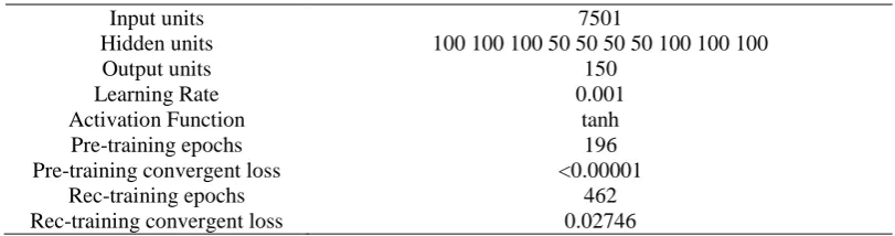
was then transformed to frequency domain, where spectrum components that have high amplitude values were taken and calculated to estimate 𝑓_𝑖. This results in the estimation of 𝑁 = 50.Then we built a 10 layers DNN model to estimate 𝐴_𝑖, 𝑓_𝑖 and 𝜃_𝑖. Some key hyper-parameters of DNN is listed below in table 1, where after 196 epochs of Pre-training, the loss value of second step was around 0.00001.

Table 1. Hyper-parameters of a ten layer multilayer perceptron.

Input units 7501

Hidden units 100 100 100 50 50 50 50 100 100 100

Output units 150

Learning Rate 0.001

Activation Function tanh

Pre-training epochs 196

Pre-training convergent loss <0.00001

Rec-training epochs 462

Rec-training convergent loss 0.02746

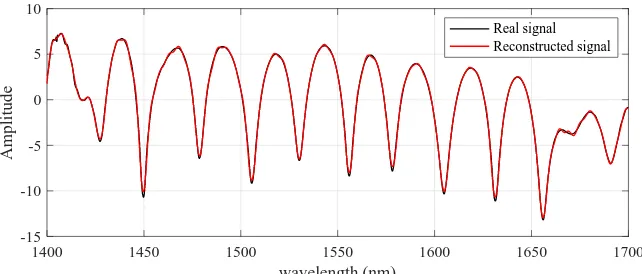
Figure 2. Comparison between real signal and reconstructed signal.

Conclusions

This paper proposes a new method that combines Deep Neural Network (DNN) and Fourier series theory to accurately model and identify complex nonlinear system with multiple parameters. The DNN with 10 layers is constructed such that it can model any nonlinear system with complex relationship between input and output, and the parameters identification is performed by the trained neural networks. The proposed method has been applied to a nonlinear system with signals measured by interferometric fiber sensors. Experimental results demonstrate that the DNN can accurately model the nonlinear system and identify the corresponding parameters, leading to a solution to complex nonlinear system approximation with minimized error.

References

[1] S. Wang, and J. Hu. A blind system identification approach to cancelable fingerprint templates. Pattern Recognition 54 (2016) 14-22.

[2] Y. Huang, L. Gao, and et al. An application of evolutionary system identification algorithm in modelling of energy production system. Measurement 114 (2018) 122-131.

[3] Y. Naung, A. Schagin, and et al. Implementation of data driven control system of DC motor by using system identification process. In 2018 IEEE Conference of Russian Young Researchers in Electrical and Electronic Engineering (EIConRus) (2018) 1801-1804.

[4] Y. H. Aleed, and T. A. Tutunji. RC helicopter modeling using re-engineering and system identification. In 2017 14th International Multi-Conference on Systems, Signals & Devices (SSD) (2017) 151-156.

[5] A. Mauroy, and J. Goncalves. Linear identification of nonlinear systems: A lifting technique based on the Koopman operator. In 2016 IEEE 55th Conference on Decision and Control (CDC) (2016) 6500-6505.

[6] S. Zhang, Y. Hui, and R. Chi. Data-driven adaptive iterative learning control based on a local dynamic linearization. In 2018 IEEE 7th Data Driven Control and Learning Systems Conference (DDCLS) (2018) 184-188.

[7] K. Yoshinaga, and et al. Approximate feedback linearization for nonlinear systems. In 2018 15th International Conference on Electrical Engineering/Electronics, Computer, Telecommunications and Information Technology (ECTI-CON) (2018) 415-420.

[8] H. K. Khalil, and J. W. Grizzle. Nonlinear Systems. Upper Saddle River, NJ: Prentice hall, 2002. pp. 1-3.

1400 1450 1500 1550 1600 1650 1700

wavelength (nm)

-15 -10 -5 0 5 10

A

m

p

li

tu

d

e

[9] K.J. Nidhil, S. Sreeraj, B. Vijay, and V. Bagyaveereswaran. System identification using artificial neural network. In 2015 International Conference on Circuits, Power and Computing Technologies [ICCPCT-2015] (2015) 1-4.

[10] H. Shu, X. Wang, and Z. Huang. Identification of multivariate system based on PID neural network. In 2015 Sixth International Conference on Intelligent Control and Information Processing (ICICIP) (2015) 199-202.

[11] M. Lopez, and W. Yu. Nonlinear system modeling using convolutional neural networks. In 2017 14th International Conference on Electrical Engineering, Computing Science and Automatic Control (CCE) (2017) 1-5.

[12] J. Vargas, E.Grzeidak, and S. CA Alfaro. Identification of unknown nonlinear systems based on multilayer neural networks and Lyapunov theory. In 2016 IEEE Symposium Series on Computational Intelligence (SSCI) (2016) 1-7.

[13] D. E. Rumelhart, G. E. Hinton, and R. J. Williams. Learning representations by back-propagating errors. Nature 323 (1986) 533–536.

[14] Y. Huang, S. Sun, X. Duan,Z. Chen. A study on Deep Neural Networks framework. 2016 IEEE Advanced Information Management, Communicates, Electronic and Automation Control Conference (IMCEC) (2016) 1-4.

[15] M. A. Nielsen, Neural Networks and Deep Learning, Determination Press, 2015, pp.39-53.

[16] N. Nagabushan, N. Satish, S. Raghuram. Effect of injected noise in Deep Neural Networks. 2016 IEEE International Conference on Computational Intelligence and Computing Research (ICCIC) (2016)1-2.

[17] H. Liu, D. Wang, J. Liu, and S. Liu. Range tunable optical fiber micro-Fabry–Pérot interferometer for pressure sensing, IEEE Photonics Technol. Lett. 28(4), 402–405 (2016).

[18] X. Fu, P. Lu, W. Ni, H. Liao, D. Liu, and J. Zhang. Phase demodulation of interferometric fiber sensor based on fast Fourier analysis. Vol. 25, No. 18, OPTICS EXPRESS 21094 (2017) 1-3.

[19] L. Gounaridis, P. Groumas, E. Schreuder, R. Heideman, H. Avramopoulos, and C. Kouloumentas. New set of design rules for resonant refractive index sensors enabled by FFT based processing of the measurement data. Optical Express 24(7) (2016) 7611–7632.