R E S E A R C H
Open Access
Relaxed alternating CQ algorithms for the
split equality problem in Hilbert spaces
Hai Yu
1*and Fenghui Wang
1*Correspondence: [email protected] 1Department of Mathematics,
Luoyang Normal University, Luoyang, P.R. China
Abstract
In this paper, we are concerned with the split equality problem (SEP) in Hilbert spaces. By converting it to a coupled fixed-point equation, we propose a new algorithm for solving the SEP. Whenever the convex sets involved are level sets of given convex functionals, we propose two new relaxed alternating algorithms for the SEP. The first relaxed algorithm is shown to be weakly convergent and the second strongly convergent. A new idea is introduced in order to prove strong convergence of the second relaxed algorithm, which gives an affirmative answer to Moudafi’s question. Finally, preliminary numerical results show the efficiency of the proposed algorithms.
MSC: 47J25; 47J20; 49N45; 65J15
Keywords: Split feasibility problem; Split equality problem; Relaxed alternating method
1 Introduction
The split feasibility problem (SFP) was first introduced by Censor and Elfving [5]. It models various inverse problems arising from phase retrievals and medical image reconstruction [3]. More specifically, the SFP requires to find a pointx∈H1satisfying the property
x∈C and Ax∈Q, (1.1)
whereCandQare nonempty, closed and convex subsets of real Hilbert spacesH1andH2,
respectively, andA:H1→H2is a bounded linear operator.
Various iterative methods have been constructed to solve the SFP (1.1); see [3–5,16, 19,20,22–25,28]. One of the well-known methods appearing in the literature for solving the SFP is Byrne’s CQ algorithm [3,4], which generates a sequence{xn}by the recursive
procedure
xn+1=PC
xn–γA∗(I–PQ)Axn
, (1.2)
whereγ ∈(0,A22),PCandPQare projections ontoCandQ, respectively,Idenotes the
identity operator, andA∗denotes the adjoint ofA. The SFP can be also solved by a different method [17,27], namely
xn+1=xn–γ
(I–PC)xn+A∗(I–PQ)Axn
, (1.3)
whereγ is a properly chosen parameter. In Hilbert spaces, both (1.2) and (1.3) converge weakly to a solution of the SFP whenever such a solution exists.
Recently, Moudafi [11] introduced the split equality problem (SEP):
Find x∈C,y∈Q such that Ax=By, (1.4)
whereH1,H2,H3are real Hilbert spaces,C⊆H1,Q⊆H2are two nonempty, closed and
convex subsets, and A:H1→H3,B:H2→H3 are two bounded linear operators. It is
clear that the SEP is more general than the SFP. As a matter of fact, ifB=IandH3=H2,
then the SEP (1.4) reduces to the SFP (1.1). Algorithms for solving the SEP have received great attention; see, for instance, [6,7,10–12,14,18]. Among these works, Moudafi [11] introduced the alternating CQ-algorithm (ACQA), namely
⎧ ⎨ ⎩
xn+1=PC(xn–γnA∗(Axn–Byn)),
yn+1=PQ(yn+γnB∗(Axn+1–Byn)).
(1.5)
It is shown that the sequence{(xn,yn)}produced by ACQA converges weakly to a solution
of (1.4) provided that the solution setS={(x,y)∈C×Q|Ax=By}is nonempty and{γn}is
a positive nondecreasing sequence such thatγn∈(,min(A12,B12) –) for a small enough > 0.
However, the ACQA might be hard to implement wheneverPC orPQfails to have a
closed-form expression. A typical example of such a situation is the level set of convex functions. Indeed, Moudafi [10] considered the case whenCandQare level sets:
C= x∈H1|c(x)≤0
(1.6)
and
Q= y∈H2|q(y)≤0
, (1.7)
wherec:H1→Randq:H2→Rare two convex and subdifferentiable functions onH1
andH2, respectively. Here the subdifferential operators∂cand∂qofcandqare assumed
to be bounded, i.e., bounded on bounded sets. In this case, it is known that the associated projections are very hard to calculate. To overcome this difficulty, Moudafi [10] presented the relaxed alternating CQ-algorithm (RACQA):
⎧ ⎨ ⎩
xn+1=PCn(xn–γA∗(Axn–Byn)),
yn+1=PQn(yn+γB∗(Axn+1–Byn)).
(1.8)
whereγ ∈(0,min(A12,B12)),{Cn}and{Qn}are two sequences of closed convex sets
de-fined by
Cn= x∈H1|c(xn) +ξn,x–xn ≤0
, ξn∈∂c(xn), (1.9)
and
Qn= y∈H2|q(yn) +ηn,y–yn ≤0
SinceCnandQnare clearly half-spaces, the associated projections thus have closed form
expressions. This indicates that the implementation of RACQA is very easy. Under suitable conditions, Moudafi [10] proved that the sequence{(xn,yn)}generated by the RACQA
converges weakly to a solution of (1.4). Meanwhile, he raised the following open question in [10].
Question 1.1 Is there any strong convergence theorem of an alternating algorithm for the SEP (1.4) in real Hilbert spaces?
Motivated by the works mentioned above, we continue to study the SEP. We will treat the SEP in a different way. Indeed, we will prove that the SEP amounts to solving the coupled fixed point equation:
⎧ ⎨ ⎩
x=x–τ[(x–PCx) +A∗(Ax–By)],
y=y–τ[(y–PQy) –B∗(Ax–By)],
(1.11)
whereτ is a positive real number. This equation enables us to propose a new algorithm for solving the SEP. We also consider the case when the convex sets involved are level sets of given convex functionals. Inspired by (1.11) and the relaxed projection algorithm, we propose two new relaxed alternating algorithms for the SEP governed by level sets, which present an affirmative answer to Moudafi’s question. Finally, we give numerical results for the split equality problem to demonstrate the feasibility and efficiency of the proposed algorithms.
2 Preliminaries
Throughout this paper, we always assume thatH is a real Hilbert space with the inner product·,· and norm · . We denote byIthe identity operator onH, and byFix(T) the set of the fixed points of an operatorT. The notation→stands for strong convergence andstands for weak convergence.
Definition 2.1([2,4]) LetT:H→Hbe an operator. ThenT is (1) nonexpansive if
Tx–Ty ≤ x–y, ∀x,y∈H;
(2) firmly nonexpansive if
Tx–Ty2≤ x–y2–(I–T)x– (I–T)y2, ∀x,y∈H.
LetCbe a nonempty, closed and convex subset ofH. For anyx∈H, the projection onto Cis defined as
PCx=argmin y–x |y∈C
.
The projectionPChas the following well-known properties.
(2) PCis nonexpansive;
(3) PCis firmly nonexpansive;
(4) PCx–PCy,x–y ≥ PCx–PCy2.
Definition 2.3 LetT :H→Hbe an operator withFix(T)=∅. ThenI–T is said to be demiclosed at zero, if, for any{xn}inH, the following implication holds:
xnx and (I–T)xn→0 ⇒ x∈Fix(T).
It is well known that ifTis a nonexpansive operator, thenI–T is demiclosed at zero. Since the projectionPCis nonexpansive, thenI–PCis demiclosed at zero.
Definition 2.4 Letλ∈(0, 1) andf :H→(–∞, +∞] be a proper function. (1) f is convex if
fλx+ (1 –λ)y≤λf(x) + (1 –λ)f(y), ∀x,y∈H.
(2) A vectoru∈His a subgradient off at a pointxif
f(y)≥f(x) +u,y–x , ∀y∈H.
(3) The set of all subgradients off atx, denoted by∂f(x), is called the subdifferential off.
To prove our main results, we need the following lemmas.
Lemma 2.5 For all x,y∈H,we have
x+y2≤ y2+ 2x,x+y .
Lemma 2.6([21]) Let{an}be a sequence of nonnegative real numbers such that
an+1≤(1 –γn)an+γnδn, n≥0,
where{γn}is a sequence in(0, 1)and{δn}is a sequence inRsuch that
(1) ∞n=0γn=∞;
(2) lim supn→∞δn≤0or
∞
n=0|δnγn|<∞.
Then,limn→∞an= 0.
3 A new alternating CQ-algorithm
In what follows, we always assume that the solution set of the SEP is nonempty, i.e., S={(x,y)∈C×Q|Ax=By} =∅. In order to solve problem (1.4), we need the following lemma, which has as a key role in later developments.
Lemma 3.1 An element(x,y)∈H1×H2solves(1.4)if and only if it solves the fixed point
Proof If (x,y) solves (1.4), thenx=PCx,y=PQyandAx=By. It is obvious that the fixed
point equation (1.11) holds.
To see the converse, let (x,y) be a solution of equation (1.11). Then,
⎧ ⎨ ⎩
(x–PCx) +A∗(Ax–By) = 0,
(y–PQy) –B∗(Ax–By) = 0.
(3.1)
Choosing any (˜x,˜y)∈S, we get
0 =(x–PCx) +A∗(Ax–By),x–x˜
=x–PCx,x–x˜ +Ax–By,Ax–Ax˜ ,
and
0 =(y–PQy) –B∗(Ax–By),y–y˜
=y–PQy,y–y˜ –Ax–By,By–By˜ .
Adding the above two equalities, we have
0 =x–PCx,x–x˜ +y–PQy,y–˜y +Ax–By2
=x–PCx,x–PCx +x–PCx,PCx–x˜ +y–PQy,y–PQy
+y–PQy,PQy–y˜ +Ax–By2
≥ x–PCx2+y–PQy2+Ax–By2.
Thus,x=PCx,y=PQyandAx=By. That is, (x,y) solves (1.4), and the proof is complete.
Applying Lemma3.1, we introduce a new alternating CQ-algorithm for the SEP (1.4).
Algorithm 3.2 Let (x0,y0)∈H1×H2be arbitrary. Given (xn,yn), construct (xn+1,yn+1) via
the formula
⎧ ⎨ ⎩
xn+1=xn–τ[(xn–PCxn) +A∗(Axn–Byn)],
yn+1=yn–τ[(yn–PQyn) –B∗(Axn+1–Byn)],
(3.2)
where 0 <τ< (1 +c)–1withc=max(A2,B2).
Theorem 3.3 Let{(xn,yn)}be the sequence generated by Algorithm3.2.Then{(xn,yn)}
con-verges weakly to a solution of the SEP(1.4).
Proof Let (x∗,y∗)∈S. Thenx∗∈C,y∗∈QandAx∗=By∗. In view of (3.2), Lemma2.2and Young’s inequality, we conclude that
xn+1–x∗ 2
=xn–x∗
2
– 2τ(xn–PCxn) +A∗(Axn–Byn),xn–x∗
+τ2(xn–PCxn) +A∗(Axn–Byn)
≤xn–x∗
2
– 2τxn–PCxn,xn–x∗
– 2τAxn–Byn,Axn–Ax∗
+τ21 +A2xn–PCxn2+
1 + 1 A2
A∗(Axn–Byn)2
≤xn–x∗
2
– 2τxn–PCxn2– 2τ
Axn–Byn,Axn–Ax∗
+τ21 +A2xn–PCxn2+Axn–Byn2
.
Similarly, we obtain
yn+1–y∗ 2
=yn–y∗
2
– 2τ(yn–PQyn) –B∗(Axn+1–Byn),yn–y∗
+τ2(yn–PQyn) –B∗(Axn+1–Byn)
2
≤yn–y∗
2
– 2τyn–PQyn,yn–y∗
+ 2τAxn+1–Byn,Byn–By∗
+τ21 +B2yn–PQyn2+
1 + 1 B2
B∗(Axn+1–Byn)
2
≤yn–y∗2– 2τyn–PQyn2+ 2τ
Axn+1–Byn,Byn–By∗
+τ21 +B2yn–PQyn2+Axn+1–Byn2
.
On the other hand, we have
2Axn–Byn,Axn–Ax∗
=Axn–Byn2+Axn–Ax∗2–Byn–Ax∗2
=Axn–Byn2+Axn–Ax∗2–Byn–By∗2
and
2Axn+1–Byn,Byn–By∗
= –Axn+1–Byn2–Byn–By∗2+Axn+1–By∗2
= –Axn+1–Byn2–Byn–By∗2+Axn+1–Ax∗2.
Altogether, we have
xn+1–x∗2≤xn–x∗2–τ
2 –1 +A2τxn–PCxn2–τAxn–Ax∗2
–τ1 –1 +A2τAxn–Byn2+τByn–By∗2
≤xn–x∗
2
–τ2 – (1 +c)τxn–PCxn2–τAxn–Ax∗
2
–τ1 – (1 +c)τAxn–Byn2+τByn–By∗
2
and
yn+1–y∗ 2
≤yn–y∗
2
–τ2 –1 +B2τyn–PQyn2+τAxn+1–Ax∗ 2
–τ1 –1 +B2τAxn+1–Byn2–τByn–By∗
≤yn–y∗
2
–τ2 – (1 +c)τyn–PQyn2+τAxn+1–Ax∗ 2
–τ1 – (1 +c)τAxn+1–Byn2–τByn–By∗
2
.
Adding the two last inequalities, we obtain
xn+1–x∗2
+yn+1–y∗ 2
≤xn–x∗
2
+yn–y∗
2
–τAxn–Ax∗
2
+τAxn+1–Ax∗ 2
–τ2 – (1 +c)τxn–PCxn2+yn–PQyn2
–τ1 – (1 +c)τAxn–Byn2+Axn+1–Byn2
. (3.3)
Let Γn(x∗,y∗) =xn –x∗2 +yn– y∗2 –τAxn –Ax∗2. Then τAxn –Ax∗2 ≤ τA2x
n–x∗2, which implies Γn
x∗,y∗≥1 –τA2xn–x∗
2
+yn–y∗
2
≥0. (3.4)
In view of (3.3), we obtain the following inequality:
Γn+1
x∗,y∗≤Γn
x∗,y∗–τ2 – (1 +c)τxn–PCxn2+yn–PQyn2
–τ1 – (1 +c)τAxn–Byn2+Axn+1–Byn2
. (3.5)
This, together with (3.4), implies that the sequence{Γn(x∗,y∗)}is bounded and converges
to some finite limitγ(x∗,y∗). By passing to the limit in (3.5) and by taking into account the assumption onτ, we finally obtain
lim
n→+∞xn–PCxn=nlim→∞yn–PQyn= 0 (3.6)
and
lim
n→∞Axn–Byn=nlim→∞Axn+1–Byn= 0. (3.7)
We next prove that any weak cluster point of the sequence{(xn,yn)}is a solution of the
SEP (1.4). Since{Γn(x∗,y∗)}is bounded, in view of (3.4), the sequences{xn}and{yn}are also
bounded. Letx¯andy¯be weak cluster points of the sequences{xn}and{yn}, respectively.
Without loss of generality, we assume thatxnx¯andyny¯. SinceI–PCandI–PQare
demiclosed at zero, from (3.6), we obtainx¯=PCx¯andy¯=PCy¯, i.e.,x¯∈Candy¯∈Q. On
the other hand, sincexnx¯andyny¯, we deduce thatAxn–BynAx¯–B¯y. The weak
lower semicontinuity of the squared norm implies
Ax¯–By¯2≤lim inf
n→∞ Axn–Byn
2= 0,
We finally show the weak convergence of the sequence{(xn,yn)}. Assume on the contrary
that (xˆ,yˆ) is another weak cluster point of{(xn,yn)}. By the definition ofΓn, we have
Γn(¯x,y¯) =Γn(ˆx,ˆy) +¯x–xˆ2+¯y–yˆ2–τAx¯–Axˆ2
+ 2xn–xˆ,xˆ–x¯ + 2yn–yˆ,yˆ–y¯ – 2τAxn–Axˆ,Axˆ–Ax¯ .
By passing to the limit in the above, we obtain
γ(x¯,y¯) =γ(xˆ,yˆ) +¯x–xˆ2+¯y–yˆ2–τAx¯–Axˆ2,
γ(ˆx,yˆ) =γ(¯x,y¯) +¯x–xˆ2+¯y–yˆ2–τAx¯–Axˆ2.
By adding the last two equalities, we obtain
1 –τA2¯x–xˆ2+¯y–yˆ2≤0,
which clearly yieldsx¯=xˆandy¯=yˆ. This in particular implies that the weak cluster point of the sequence{(xn,yn)}is unique. Consequently, the whole sequence{(xn,yn)}converges
weakly to a solution of problem (1.4).
4 A relaxed alternating CQ-algorithm
WhenCandQare level sets, the projections in Algorithm3.2might be hard to be im-plemented (see [1,8,9,13,25,26]). To overcome this difficulty, we propose a relaxed al-ternating CQ-algorithm, which is inspired by methods (1.8) and (3.2). In what follows, we will treat the SEP (1.4) under the following assumptions:
(A1) The setsCandQare given by (1.6) and (1.7), respectively.
(A2) For anyx∈H1andy∈H2, at least one subgradientξ∈∂c(x)andη∈∂q(y)can be
calculated.
We now present a new relaxed alternative CQ algorithm for solving the SEP (1.4).
Algorithm 4.1 Let (x0,y0) be arbitrary. Given (xn,yn), construct (xn+1,yn+1) via the
for-mula
⎧ ⎨ ⎩
xn+1=xn–τ[(xn–PCnxn) +A∗(Axn–Byn)], yn+1=yn–τ[(yn–PQnyn) –B∗(Axn+1–Byn)],
(4.1)
where 0 <τ < (1 +c)–1 withc=max(A2,B2), andC
nandQn are given as (1.9) and
(1.10), respectively.
Remark4.2 By the definition of the subgradient, it is clear thatC⊆CnandQ⊆Qnfor all
n≥0. SinceCnandQnare both half-spaces, the projections ontoCnandQncan be easily
calculated. Thus Algorithm4.1is easily implementable.
Theorem 4.3 Let{(xn,yn)}be the sequence generated by Algorithm4.1.Then{(xn,yn)}
Proof Taking (x∗,y∗)∈S, i.e.,x∗∈C(and thusx∗∈Cn),y∗∈Q(and thusy∗ ∈Qn), we
haveAx∗=By∗. LetΓn(x∗,y∗) =xn–x∗2+yn–y∗2–τAxn–Ax∗2. Similarly as in
Theorem3.3, we obtain the following inequality:
Γn+1
x∗,y∗≤Γn
x∗,y∗–τ2 – (1 +c)τxn–PCnxn2+yn–PQnyn2
–τ1 – (1 +c)τAxn–Byn2+Axn+1–Byn2
. (4.2)
In addition, we have
Γn
x∗,y∗≥1 –τA2xn–x∗2+yn–y∗2≥0. (4.3)
It follows that the sequence{Γn(x∗,y∗)}is bounded and converges to some finite limit γ(x∗,y∗), which yields
lim
n→∞xn–PCnxn=nlim→∞yn–PQnyn= 0 (4.4)
and
lim
n→∞Axn–Byn=nlim→∞Axn+1–Byn= 0. (4.5)
From (4.1), we obtain
xn+1–xn=τ
(xn–PCnxn) +A
∗(Ax
n–Byn)
≤τxn–PCnxn+AAxn–Byn
→0
and
yn+1–yn=τ
(yn–PQnyn) –B∗(Axn+1–Byn)
≤τyn–PQnyn+BAxn+1–Byn
→0.
We next prove that any weak cluster point of the sequence{(xn,yn)}is a solution of the
SEP (1.4). Since{Γn(x∗,y∗)}is bounded, in view of (4.3), the sequences{xn}and{yn}are also
bounded. Letx¯andy¯be weak cluster points of the sequences{xn}and{yn}, respectively.
Without loss of generality, we assume thatxnx¯ andyny¯. Since∂cis bounded on
bounded sets, there is a constantδ1> 0 such thatξn ≤δ1for alln≥0. From (4.1), we
have
xn–
1
τ(xn–xn+1) +A
∗(Ax
n–Byn) =PCnxn∈Cn.
This implies that
c(xn) +
ξn, –
1
τ(xn–xn+1) +A
∗(Ax
n–Byn)
Thus
c(xn)≤
ξn,
1
τ(xn–xn+1) –A
∗(Ax
n–Byn)
≤δ1
τ xn–xn+1+δ1AAxn–Byn →0.
The weak lower semicontinuity ofcleads to
c(¯x)≤lim inf
n→∞ c(xn)≤0,
and thereforex¯∈C. Likewise, since∂qis bounded on bounded sets, there is a constant δ2> 0 such thatηn ≤δ2for alln≥0. From (4.1), we have
yn–
1
τ(yn–yn+1) –B
∗(Ax
n+1–Byn) =PQnyn∈Qn.
This implies that
q(yn) +
ηn, –
1
τ(yn–yn+1) –B
∗(Ax
n+1–Byn)
≤0.
Hence
q(yn)≤
ηn,
1
τ(yn–yn+1) +B
∗(Ax
n+1–Byn)
≤δ2
τ yn–yn+1+δ2BAxn+1–Byn →0.
Again, the weak lower semicontinuity ofqleads to
q(¯y)≤lim inf
n→∞ q(yn)≤0,
and thereforey¯∈Q. Furthermore, the weak convergence of{Axn–Byn}toAx¯–By¯and the
weak lower semicontinuity of the squared norm imply
Ax¯–By¯2≤lim inf
n→∞ Axn–Byn
2= 0.
Hence (¯x,y¯)∈S.
The proof of the uniqueness of the weak cluster point is analogous to that of Theo-rem3.3. Therefore, the whole sequence{(xn,yn)}converges weakly to a solution of
prob-lem (1.4). This completes the proof.
5 A strongly convergent algorithm
Algorithm 5.1 Let (u,v)∈H1×H2be fixed and start with an initial guess (x0,y0)∈H1×
H2. Given (xn,yn), construct (xn+1,yn+1) via the formula
⎧ ⎪ ⎪ ⎪ ⎪ ⎪ ⎨ ⎪ ⎪ ⎪ ⎪ ⎪ ⎩
un=xn–τ[(xn–PCnxn) +A∗(Axn–Byn)], xn+1=αnu+ (1 –αn)un,
vn=yn–τ[(yn–PQnyn) –B∗(Axn+1–Byn)], yn+1=αnv+ (1 –αn)vn,
(5.1)
where{αn}is a sequence in [0, 1], 0 <τ < (1 +c)–1 withc=max(A2,B2), andCnand
Qnare given as (1.9) and (1.10), respectively.
Theorem 5.2 Let{(xn,yn)}be the sequence generated by Algorithm5.1.If{αn}satisfies the
following conditions:
lim
n→∞αn= 0 and
∞
n=1
αn=∞,
then {(xn,yn)} converges strongly to a solution(x∗,y∗)of the SEP (1.4), where(x∗,y∗) =
PS(u,v).
Proof Since (x∗,y∗) =PS(u,v)∈S, we havex∗∈C(and thusx∗∈Cn),y∗∈Q(and thus
y∗∈Qn),Ax∗=By∗. In what follows, we divide the proof into four steps.
Step1. We prove that the sequences{xn}and{yn}are bounded. By the same argument
as in the proof of Theorem3.3, we arrive at
un–x∗2+vn–y∗2
≤xn–x∗
2
+yn–y∗
2
–τAxn–Ax∗
2
+τAxn+1–Ax∗ 2
–τ2 – (1 +c)τxn–PCnxn
2+y
n–PQnyn
2
–τ1 – (1 +c)τAxn–Byn2+Axn+1–Byn2
. (5.2)
In view of (5.1) and the convexity of the squared norm, we obtain
xn+1–x∗ 2
+yn+1–y∗ 2
=αn
u–x∗+ (1 –αn)
un–x∗
2
+αn
v–y∗+ (1 –αn)
vn–y∗
2
≤αnu–x∗
2
+ (1 –αn)un–x∗
2
+αnv–y∗
2
+ (1 –αn)vn–y∗
2
=αnu–x∗
2
+v–y∗2+ (1 –αn)un–x∗
2
+vn–y∗
2
.
This, along with (5.2), implies that
xn+1–x∗2+yn+1–y∗2
≤αnu–x∗
2
+v–y∗2+ (1 –αn)xn–x∗
2
+yn–y∗
2
–τAxn–Ax∗
2
–τ2 – (1 +c)τxn–PCnxn
2+y
n–PQnyn
2
–τ1 – (1 +c)τAxn–Byn2+Axn+1–Byn2
≤αnu–x∗
2
+v–y∗2+τAxn+1–Ax∗ 2
+ (1 –αn)xn–x∗
2
+yn–y∗
2
–τAxn–Ax∗
2
–τ2 – (1 +c)τxn–PCnxn
2+y
n–PQnyn
2
–τ1 – (1 +c)τAxn–Byn2+Axn+1–Byn2
. (5.3)
Now, by setting
Γn
x∗,y∗=xn–x∗
2
+yn–y∗
2
–τAxn–Ax∗
2
,
we have
Γn
x∗,y∗≥1 –τA2xn–x∗
2
+yn–y∗
2
≥0. (5.4)
In view of (5.3), we conclude that
Γn+1
x∗,y∗≤(1 –αn)Γn
x∗,y∗+αnu–x∗2+v–y∗2
– (1 –αn)
τ2 – (1 +c)τxn–PCnxn2+yn–PQnyn2
+τ1 – (1 +c)τAxn–Byn2+Axn+1–Byn2
.
This implies
Γn+1
x∗,y∗≤(1 –αn)Γn
x∗,y∗+αnu–x∗
2
+v–y∗2 ≤max Γn
x∗,y∗,u–x∗2+v–y∗2. By induction, we obtain
Γn+1
x∗,y∗≤max Γ0
x∗,y∗,u–x∗2+v–y∗2
for alln≥0. This implies that the sequence{Γn(x∗,y∗)}is bounded. Hence, in view of (5.4),
the sequences{xn}and{yn}are bounded, too.
Step2. We show that the following inequality holds:
Γn+1
x∗,y∗≤(1 –αn)Γn
x∗,y∗+αnδn, (5.5)
where
δn= 2
u–x∗,xn+1–x∗
+v–y∗,yn+1–y∗
–(1 –αn) αn
τ2 – (1 +c)τxn–PCnxn
2+y
n–PQnyn
2
+τ1 – (1 +c)τAxn–Byn2+Axn+1–Byn2
Indeed, by Lemma2.5, we have
xn+1–x∗2+yn+1–y∗2
=αn
u–x∗+ (1 –αn)
un–x∗2+αn
v–y∗+ (1 –αn)
vn–y∗2
≤(1 –αn)un–x∗
2
+ 2αn
u–x∗,xn+1–x∗
+ (1 –αn)vn–y∗
2
+ 2αn
v–y∗,yn+1–y∗
= (1 –αn)un–x∗
2
+vn–y∗
2
+ 2αn
u–x∗,xn+1–x∗
+v–y∗,yn+1–y∗
.
Again from (5.2), we obtain
xn+1–x∗ 2
+yn+1–y∗ 2
≤(1 –αn)xn–x∗
2
+yn–y∗
2
–τAxn–Ax∗
2
+τAxn+1–By∗ 2
–τ2 – (1 +c)τxn–PCnxn
2+y
n–PQnyn
2
–τ1 – (1 +c)τAxn–Byn2+Axn+1–Byn2
+ 2αn
u–x∗,xn+1–x∗
+v–y∗,yn+1–y∗
≤(1 –αn)xn–x∗
2
+yn–y∗
2
–τAxn–Ax∗
2
+τAxn+1–By∗ 2
– (1 –αn)
τ2 – (1 +c)τxn–PCnxn2+yn–PQnyn2
+τ1 – (1 +c)τAxn–Byn2+Axn+1–Byn2
+ 2αn
u–x∗,xn+1–x∗
+v–y∗,yn+1–y∗
.
This implies
Γn+1
x∗,y∗≤(1 –αn)Γn
x∗,y∗ – (1 –αn)
τ2 – (1 +c)τxn–PCnxn2+yn–PQnyn2
+τ1 – (1 +c)τAxn–Byn2+Axn+1–Byn2
+ 2αn
u–x∗,xn+1–x∗
+v–y∗,yn+1–y∗
= (1 –αn)Γn
x∗,y∗+αn
2u–x∗,xn+1–x∗
+v–y∗,yn+1–y∗
–(1 –αn) αn
τ2 – (1 +c)τxn–PCnxn2+yn–PQnyn2
+τ1 – (1 +c)τAxn–Byn2+Axn+1–Byn2
.
Hence, the desired inequality follows at once.
Step3. We show thatlim supn→∞δnis finite. Since{xn}and{yn}are bounded, we have δn≤2
u–x∗,xn+1–x∗
+v–y∗,yn+1–y∗
This implies thatlim supn→∞δn<∞. We now showlim supn→∞δn≥–1 by contradiction.
If we assume on the contrary thatlim supn→∞δn< –1, then there existsn0such thatδn≤
–1 for alln≥n0. It then follows from (5.5) that
Γn+1
x∗,y∗≤(1 –αn)Γn
x∗,y∗+αnδn
≤(1 –αn)Γn
x∗,y∗–αn
=Γn
x∗,y∗–αn
Γn
x∗,y∗+ 1 ≤Γn
x∗,y∗–αn
for alln≥n0. By induction, we have
Γn+1
x∗,y∗≤Γn0
x∗,y∗–
n
i=n0 αi.
Since ∞i=n0αi=∞, there existsN>n0 such that
N
i=n0αi>Γn0(x∗,y∗). Therefore, we have
ΓN+1
x∗,y∗≤Γn0
x∗,y∗–
N
i=n0 αi< 0,
which clearly contradicts the fact that Γn(x∗,y∗) is a nonnegative real sequence. Thus,
lim supn→∞δn≥–1 and it is finite.
Step4. We show thatlim supn→∞δn≤0 and{(xn,yn)}converges strongly to (x∗,y∗). Since
lim supn→∞δnis finite, we can take a subsequence{nk}such that
lim sup
n→∞ δn=klim→∞δnk = lim
k→∞
2u–x∗,xnk+1–x
∗+v–y∗,y
nk+1–y
∗
–(1 –αnk)
αnk
τ2 – (1 +c)τxnk–PCnkxnk
2+y
nk–PQnkynk
2
+τ1 – (1 +c)τAxnk–Bynk
2+Ax
nk+1–Bynk
2. (5.6)
Sinceu–x∗,xn+1–x∗ andv–y∗,yn+1–y∗ are bounded, without loss of generality, we
may assume the existence of the limits
lim
k→∞
u–x∗,xnk+1–x
∗ and lim
k→∞
v–y∗,ynk+1–y
∗.
Hence, from (5.6), the following limit also exists:
lim
k→∞
(1 –αnk)
αnk
τ2 – (1 +c)τxnk–PCnkxnk
2+y
nk–PQnkynk
2
+τ1 – (1 +c)τAxnk–Bynk
2+Ax
nk+1–Bynk
Sincelimk→∞αnk= 0, we getlimk→∞
1–αnk
αnk =∞. This implies that
lim
k→∞
τ2 – (1 +c)τxnk–PCnkxnk
2+y
nk–PQnkynk
2
+τ1 – (1 +c)τAxnk–Bynk
2+Ax
nk+1–Bynk
2= 0.
So, by taking into account the assumption onτ, we have
lim
k→∞xnk–PCnkxnk= lim
k→∞ynk–PQnkynk= 0 and
lim
k→∞Axnk–Bynk= lim
k→∞Axnk+1–Bynk= 0. From (5.1), we deduce that
lim
k→∞unk–xnk= lim
k→∞τ(xnk–PCnkxnk) +A
∗(Ax
nk–Bynk)
≤τ lim
k→∞
xnk–PCnkxnk+AAxnk–Bynk
= 0
and
lim
k→∞vnk–ynk= lim
k→∞τ(ynk–PQnkynk) –B
∗(Ax
nk+1–Bynk)
≤τ lim
k→∞
ynk–PQnkynk+BAxnk+1–Bynk
= 0.
Similarly as in the proof of Theorem4.3, we conclude that any weak cluster point of {(xnk,ynk)}belongs toS.
Since the sequences{xn}and{yn}are bounded, one gets
lim
k→∞xnk+1–xnk= lim
k→∞αnk(u–xnk) + (1 –αnk)(unk–xnk) ≤ lim
k→∞
αnku–xnk+unk–xnk
= 0
and
lim
k→∞ynk+1–ynk= lim
k→∞αnk(v–ynk) + (1 –αnk)(vnk–ynk) ≤ lim
k→∞
αnkv–ynk+vnk–ynk
= 0.
This implies that any weak cluster point of{(xnk+1,ynk+1)}also belongs toS. Without loss of generality, we assume that{(xnk+1,ynk+1)}converges weakly to (ˆx,ˆy)∈S. Now by (5.6), Lemma2.2and the fact that (x∗,y∗) =PS(u,v), we obtain
lim sup
n→∞
δn≤ lim k→∞2
u–x∗,xnk+1–x
∗+v–y∗,y
nk+1–y
∗
Applying Lemma2.6to (5.5), we havelimn→∞Γn(x∗,y∗) = 0. Finally, by (5.4), we infer that
lim
n→∞xn–x
∗= 0 and lim
n→∞yn–y ∗= 0,
which ends the proof.
6 Numerical results
In this section, we verify the feasibility and efficiency of our algorithms through an exam-ple. The whole codes are written in Matlab R2012b on a personal computer with Inter(R) Core(TM) i5-4590 CPU, 3.30 GHz and 4 GB RAM.
Example6.1 LetH1=H2=H3=R3,
A=
⎡ ⎢ ⎣
√
5 0 0
0 5 0
0 0 1
⎤ ⎥
⎦, B=
⎡ ⎢ ⎣
1 0 0
0 1 0
0 0 1
⎤ ⎥ ⎦,
C={x∈R3|x= (u,v,w)T,v2+w2– 1≤0}, andQ={y∈R3|y= (u,v,w)T,u2–v+ 5≤0}.
Findx∈C,y∈Qsuch thatAx=By.
It is easy to verify that this problem has a unique solution (¯x,y¯)∈R3×R3, wherex¯= (0, 1, 0)T,y¯= (0, 5, 0)T. In the experiments, we takeγ = 0.9×min( 1
A2,B12) in RACQA algorithm (1.8) andτ = 0.9×(1 +c)–1 withc=max(A2,B2) in Algorithm4.1. The
stopping criterion isxk+1–xk+yk+1–yk< 10–3andAxk–Byk< 10–3. The numerical
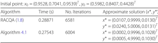
[image:16.595.167.426.501.573.2]results can be seen from Tables1–3. It is worth noting that the initial point in Table3is generated randomly. From Tables1–3, we can see that the CPU time and iteration number of Algorithm4.1are less than that of RACQA algorithm (1.8).
Table 1 Numerical results of Example6.1
Initial point:x0= (1, 1, 1)T,y0= (0, 0, 0)T
Algorithm Time (s) No. Iterations Approximate solution (x∗,y∗)
RACQA (1.8) 0.34021 7357 x∗= (0.0130, 1.000, 0.0079)T
y∗= (0.0291, 5.0008, 0.0079)T
Algorithm4.1 0.26312 5847 x∗= (0.0001, 0.9996, 0.1028)T
y∗= (0.0002, 4.9990, 0.1030)T
Table 2 Numerical results of Example6.1
Initial point:x0= (5, 5, 5)T,y0= (1, 1, 1)T
Algorithm Time (s) No. Iterations Approximate solution (x∗,y∗)
RACQA (1.8) 0.32586 7010 x∗= (0.0120, 0.9999, 0.0106)T
y∗= (0.0268, 5.0007, 0.0106)T
Algorithm4.1 0.27749 6250 x∗= (0.0003, 0.9996, 0.1028)T
[image:16.595.168.427.629.701.2]Table 3 Numerical results of Example6.1
Initial point:x0= (0.9528, 0.7041, 0.9539)T,y0= (0.5982, 0.8407, 0.4428)T
Algorithm Time (s) No. Iterations Approximate solution (x∗,y∗)
RACQA (1.8) 0.28871 6581 x∗= (0.0107, 0.9999, 0.0130)T
y∗= (0.0240, 5.0006, 0.0131)T
Algorithm4.1 0.27543 6004 x∗= (0.0002, 0.9996, 0.1028)T
y∗= (0.0005, 4.9990, 0.1030)T
Acknowledgements Not applicable.
Funding
This work was supported by the National Natural Science Foundation of China (Nos. 11301253, 11571005), Program for Science and Technology Innovation Talents in the Universities of Henan Province (Grant No. 15HASTIT013), Innovation Scientists and Technicians Troop Construction Projects of Henan Province (Grant No. CXTD20150027) and Foundation of He’nan Educational Committee (Nos. 16A520064, 15A520087).
Availability of data and materials Not applicable.
Competing interests
The authors declare that they have no competing interests.
Authors’ contributions
All authors contributed equally to the writing of this paper. All authors read and approved the final manuscript.
Publisher’s Note
Springer Nature remains neutral with regard to jurisdictional claims in published maps and institutional affiliations.
Received: 26 October 2018 Accepted: 3 December 2018 References
1. Bauschke, H.H., Borwein, J.M.: On projection algorithms for solving convex feasibility problems. SIAM Rev.38, 367–426 (1996)
2. Bauschke, H.H., Combettes, P.L.: Convex Analysis and Monotone Operator Theory in Hilbert Space. Springer, New York (2011)
3. Byrne, C.: Iterative oblique projection onto convex sets and the split feasibility problem. Inverse Probl.18, 441–453 (2002)
4. Byrne, C.: A unified treatment of some iterative algorithms in signal processing and image reconstruction. Inverse Probl.20, 103–120 (2004)
5. Censor, Y., Elfving, T.: A multiprojection algorithm using Bregman projections in a product space. Numer. Algorithms 8, 221–239 (1994)
6. Chuang, C., Du, W.: Hybrid simultaneous algorithms for the split equality problem with applications. J. Inequal. Appl. 2016(1), 198 (2016)
7. Dong, Q., He, S., Zhao, J.: Solving the split equality problem without prior knowledge of operator norms. Optimization 64(9), 1887–1906 (2015)
8. Fukushima, M.: A relaxed projection method for variational inequalities. Math. Program.35, 58–70 (1986) 9. He, B.S.: Inexact implicit methods for monotone general variational inequalities. Math. Program., Ser. A86, 199–217
(1999)
10. Moudafi, A.: A relaxed alternating CQ-algorithm for convex feasibility problems. Nonlinear Anal.79, 117–121 (2013) 11. Moudafi, A.: Alternating CQ-algorithm for convex feasibility and split fixed-point problems. J. Nonlinear Convex Anal.
15, 809–818 (2014)
12. Naraghirad, E.: On an open question of Moudafi for convex feasibility problem in Hilbert spaces. Taiwan. J. Math. 18(2), 371–408 (2014)
13. Qu, B., Xiu, N.H.: A new half-space-relaxation projection method for the split feasibility problem. Linear Algebra Appl. 428, 1218–1229 (2008)
14. Shi, L., Chen, R., Wu, Y.: Strong convergence of iterative algorithms for the split equality problem. J. Inequal. Appl. 2014(1), 478 (2014)
15. Takahashi, W.: Nonlinear Functional Analysis, Fixed Point Theory and Its Applications. Yokahama Publishers, Yokahama (2000)
16. Tang, Y., Liu, L.: Iterative methods of strong convergence theorems for the split feasibility problem in Hilbert spaces. J. Inequal. Appl.2016(1), 284 (2016)
17. Wang, F.: A new iterative method for the split common fixed point problem in Hilbert spaces. Optimization66, 407–415 (2017)
18. Wang, F.: On the convergence of CQ algorithm with variable steps for the split equality problem. Numer. Algorithms 74, 927–935 (2017)
20. Wang, F., Xu, H.K.: Cyclic algorithms for split feasibility problems in Hilbert spaces. Nonlinear Anal.74, 4105–4111 (2011)
21. Xu, H.K.: Iterative algorithms for nonlinear operators. J. Lond. Math. Soc.66, 240–256 (2002)
22. Xu, H.K.: A variable Krasnosel’skii–Mann algorithm and the multiple-set split feasibility problem. Inverse Probl.22, 2021–2034 (2006)
23. Xu, H.K.: Iterative methods for the split feasibility problem in infinite-dimensional Hilbert spaces. Inverse Probl.26, 105018 (2010)
24. Xu, H.K.: Properties and iterative methods for the lasso and its variants. Chin. Ann. Math., Ser. B35(3), 501–518 (2014) 25. Yang, Q.: The relaxed CQ algorithm solving the split feasibility problem. Inverse Probl.20, 1261–1266 (2004) 26. Yang, Q.: On variable-step relaxed projection algorithm for variational inequalities. J. Math. Anal. Appl.302, 166–179
(2005)
27. Yao, Y., Liou, Y., Postolache, M.: Self-adaptive algorithms for the split problem of the demicontractive operators. Optimization (2017).https://doi.org/10.1080/02331934.2017.1390747
28. Yu, H., Zhan, W., Wang, F.: The ball-relaxed CQ algorithms for the split feasibility problem. Optimization (2018).