M estimation in high dimensional linear model

R E S E A R C H

Open Access

M-estimation in high-dimensional linear

model

Kai Wang

_{and Yanling Zhu}

*_{Correspondence:} [email protected] 1_{School of Statistics and Applied}

Mathematics, Anhui University of Finance and Economics, Bengbu, P.R. China

Abstract

We mainly study the M-estimation method for the high-dimensional linear regression model and discuss the properties of the M-estimator when the penalty term is a local linear approximation. In fact, the M-estimation method is a framework which covers the methods of the least absolute deviation, the quantile regression, the least squares regression and the Huber regression. We show that the proposed estimator possesses the good properties by applying certain assumptions. In the part of the numerical simulation, we select the appropriate algorithm to show the good robustness of this method.

MSC: 62F12; 62E15; 62J05

Keywords: M-estimation; High-dimensionality; Variable selection; Oracle property; Penalized method

1 Introduction

For the classical linear regression modelY =Xβ +ε, we are interested in the prob-lem of variable selection and estimation, whereY= (y1,y2, . . . ,yn)T is the response

vec-tor,X= (X1,X2, . . . ,Xpn) = (x1,x2, . . . ,xn)T= (xij)n×pn is ann×pndesign matrix, andε=

(ε1,ε2, . . . ,εn)Tis a random vector. The main topic is how to estimate the coefficients

vec-torβ∈Rp_nwhenpnincreases with sample sizenand many elements ofβequal zero. We

can transfer this problem into a minimization of a penalized least squares objective func-tion

ˆ

βn=arg min

β Qn(βn), Qn(βn) =Y–Xβn

2₊

pn

j=1 pλn

|βnj|

,

where · is thel2 norm of the vector,λnis a tuning parameter, andpλn(|t|) a penalty

term. It is well known that the least squares estimation is not robust, especially when in the data there exist abnormal values or the error term has a heavy-tailed distribution.

In this paper we consider the loss function to be the least absolute deviation, i.e., we minimize the following objective function:

ˆ

βn=arg min

β Qn(βn), Qn(βn) =

1 n

n

i=1

yi–xTi βn+ pn

j=1 pλn

|βnj|

,

where the loss function is the least absolute deviation (LAD for short) that does not need the noise to obey a gaussian distribution and be more robust than a least squares estima-tion. In fact, the LAD estimation is a special case of the M-estimation, which was men-tioned by Huber (1964, 1973, 1981) [1–3] firstly and which can be obtained by minimizing the objective function

Qn(βn) =

1 n

n

i=1

ρyi–xTi βn

,

where the functionρcan be selected. For example, if we chooseρ(x) =1₂x21|x|≤c+ (c|x|–

c2/2)1|x|>c, wherec> 0, the Huber estimator can be obtained; if we chooseρ(x) =|x|q,

where 1≤q≤2,Lqestimator will be obtained, with two special cases: LAD estimator for

q= 1 and OLS estimator forq= 2. If we chooseρ(x) =αx+_{+ (1 –α)(–x)}+_{, where 0 <α< 1,} x+_{=max(x, 0), we call it a quantile regression, and we can also get the LAD estimator for} α= 1/2 especially.

Whenpnapproaches infinity asntends to infinity, we assume that the functionρ is

convex and not monotone, and the monotone functionϕis the derivative ofρ. By impos-ing the appropriate regularity conditions, Huber (1973), Portnoy (1984) [4], Welsh (1989) [5] and Mammen (1989) [6] have proved that the M-estimator enjoyed the properties of consistency and asymptotic normality, where Welsh (1989) gave the weaker condition im-posed onϕand the stronger condition onpn/n. Bai and Wu [7] further pointed out that the

condition onpncould be a part of the integrable condition imposed on the design matrix.

Moreover, He and Shao (2000) [8] studied the asymptotic properties of the M-estimator in the case of a generalized model setting and the dimensionpngetting bigger and

big-ger. Li (2011) [9] obtained the Oracle property of the non-concave penalized M-estimator in high-dimensional model with the condition ofpnlogn/n→0,p2n/n→0, and proposed

RSIS to make a variable selection by applying a rank sure independence screening method in the ultra high-dimensional model. Zou and Li (2008) [10] combined a penalized func-tion and a local linear approximafunc-tion method (LLA) to prove that the obtained estimator enjoyed good asymptotic properties, and they demonstrated that this method improved the computational efficiency of a local quadratic approximation (LQA) in a simulation.

Inspired by this, in this paper we consider the following problem:

ˆ

βn=arg min βn

Qn(βn), Qn(βn) =

1 n

n

i=1

ρyi–xTiβn

+

pn

j=1

p_λn| ˜βnj|

|βnj|, (1.1)

wherepλn(·) is the derivative of the penalized function, andβ˜n= (β˜n1,β˜n2, . . . ,β˜npn)Tis the

non-penalized estimator.

In this paper, we assume that the functionρis convex, hence the objective function is still convex and the obtained local minimizer is a global minimizer.

2 Main results

For convenience, we first give some notations. Letβ0= (β01,β02, . . . ,β0p)Tbe the true

pa-rameter. Without loss of generality, we assume the firstkncoefficients of the covariates

are nonzero, then there arepn–kncovariates with zero coefficients.β0= (β0(1)T ,β0(2)T )T,

ˆ

andλmax(Z) the minimum and maximum eigenvalue ofZ, respectively. Denote XT_nX:=D andD=D11D12

D21D22

, where D11= 1_nX(1)TX(1). Finally, we denotecn=max{|pλn(| ˜βnj|)|:β˜nj=

0, 1≤j≤pn}.

Next, we state some assumptions which will be needed in the following results. (A1) The functionρis convex onR, and its left derivative and right derivativeϕ+(·),ϕ–(·)

satisfiesϕ–(t)≤ϕ(t)≤ϕ+(t),∀t∈R.

(A2) The error termεis i.i.d, and the distribution functionFofεisatisfiesF(S) = 0, where

Sis the set of discontinuous points ofϕ.

Moreover,E[ϕ(εi)] = 0,0 <E[ϕ2(εi)] =σ2<∞, andG(t)≡E[ϕ(εi+t)] =γt+

o(|t|), whereγ> 0. Besides these, we assume thatlimt→0E[ϕ(εi+t) –ϕ(εi)]2= 0.

(A3) There exist constantsτ1,τ2,τ3,τ4 such that0 <τ1≤λmin(D)≤λmax(D)≤τ2 and 0 <τ3≤λmin(D11)≤λmax(D11)≤τ4.

(A4) λn→0(n→ ∞),pn=O(n1/2),cn=O(n–1/2).

(A5) Let zi be the transpose of the ith row vector of X(1), such that limn→∞n–

1 2×

max_1≤i≤nzT izi= 0.

It is worth mentioning that conditions (A1) and (A2) are classical assumptions for an M-estimation in a linear model, which can be found in many references, for example Bai, Rao and Wu (1992) [11] and Wu (2007) [12]. The condition (A3) is frequently used for a sparse model in the linear model regression theory, which requires that the eigenvalues of the matricesDandD11are bounded. The condition (A4) is weaker than that in previ-ous references. Under the condition (A4) we broaden the order ofpnton1/2, but Huber

(1973) and Li, Peng and Zhu (2011) [9] required thatp2

n/n→0, Portnoy (1984) required

pnlogpn/n→0, and Mammen (1989) requiredp3/2n logpn/n→0. Compared with these

results, it is obvious that our sparse condition is much weaker. The condition (A5) is the same as that in Huang, Horowitz and Ma (2008) [13], which is used to prove the asymp-totic properties of the nonzero part of M-estimation.

Theorem 2.1(Consistency of estimator) If the conditions(A1)–(A4)hold,there exists a non-concave penalized M-estimationβˆn,such that

ˆβn–β0=OP

(pn/n)1/2

.

Remark2.1 From Theorem2.1, we can see that there exists a global M-estimationβˆnif

we choose the appropriate tuning parameterλn; moreover, this M-estimation is (n/pn)1/2

-consistent. This convergence rate is the same as that in the work of Huber (1973) and Li, Peng and Zhu (2011).

Theorem 2.2(The sparse model) If the conditions(A1)–(A4)hold andλmin(D) >λmax(1_n×

n

i=1JiJiT),for the non-concave penalized M-estimationβˆnwe have

P(βˆn(2)= 0)→1.

Theorem 2.3(Oracle property) If the conditions(A1)–(A5)hold andλmin(D) >λmax(1_n×

n

i=1JiJiT),with probability converging to one,the non-concave penalized M-estimation

ˆ

βn= (βˆnT(1),βˆnT(2))Thas the following properties: (1) (The consistency of the model selection)βˆn(2)= 0; (2) (Asymptotic normality)

√

ns–1_n uT(βˆn(1)–β0(1)) =

n

i=1

n–1/2s–1_n γ–1uTD11zTiϕ(εi) +oP(1)

d

−→N(0, 1),

wheres2

n=σ2γ–1uTD–111u,anduis anykndimensional vector such thatu ≤1.

Meanwhile,ziis the transpose of theith row vector of akn×knmatrixX(1).

Remark 2.3 From Theorem2.3, the M-estimation enjoys the Oracle property, that is, the M-estimator can correctly select covariates with nonzero coefficients with proba-bility converging to one and the estimators of the nonzero coefficients has the same asymptotic distribution that they would have if the zero coefficients were known in ad-vance.

Remark2.4 In Fan and Peng (2004) [14], the authors showed that the non-concave pe-nalized M-estimation has the property of consistency with the condition p4

n/n →0,

and enjoyed the property of asymptotic normality with the condition p5

n/n→0. By

Theorems 2.1–2.3, we can see that the corresponding conditions we impose are quite weak.

3 Proofs of main results

The proof of Theorem2.1 Letαn= (pn/n)1/2+p1/2n cn. For anypn-dimensional vectoruwith

u=C, we only need to prove that there exists a great enough positive constantCsuch that

lim inf

n→∞ P

inf

u=CQn(β0+αnu) >Qn(β0)

≥1 –ε,

for anyε> 0, that is, there at least exists a local minimizerβˆnsuch that ˆβn–β0=OP(αn)

in the closed ball{β0+αnu:u ≤C}.

Firstly, by the triangle inequality we get

Qn(β0+θu) –Qn(β0)

=1 n

n

i=1

ρyi–xTi (β0+αnu)

–ρyi–xTiβ0

+

pn

j=1

p_λn| ˜βnj|

|β0j+αnuj|–|β0j|

≥1

n

n

i=1

ρyi–xTi(β0+αnu)

–ρyi–xTiβ0

–αn pn

j=1 pλn

| ˜βnj|

|uj|

whereT1=1_n

n

i=1[ρ(yi–xTi(β0+αnu)) –ρ(yi–xTiβ0)],T2= –αn

pn

j=1pλn(| ˜βnj|)|uj|.

Notic-ing that

T1= 1 n

n

i=1

ρyi–xTi(β0+αnu)

–ρyi–xTi β0

=1 n n i=1

ρεi–αnxTiu

–ρ(εi)

=1 n n i=1

–αnxTiu

0

ϕ(εi+t) –ϕ(εi)

dt–1 nαn

n

i=1

ϕ(εi)xTiu

:=T11+T12, (3.1)

whereT11=1_nni=1

–αnxT_iu

0 [ϕ(εi+t)–ϕ(εi)]dt,T12= –_n1αnni=1ϕ(εi)xTiu. Combining with

the Von-Bahr–Esseen inequality and the fact that|T12| ≤ 1_nαnu

n

i=1ϕ(εi)xi, we

in-stantly have E n i=1 ϕ(εi)xi

2 ≤n n i=1

E ϕ(εi)xi

2 =n

n

i=1

E[ϕ2(εi)xTi xi≤n2pnσ2,

hence

|T12|=OP

αnp1/2n

u=OP

p2_n/n1/2. (3.2)

Secondly forT11, letT11=

n

i=1Ain, whereAin=1_n

–αnxTiu

0 [ϕ(εi+t) –ϕ(εi)]dt, so

T11=

n

i=1

Ain–E(Ain)

+

n

i=1

E(Ain) :=T111+T112.

We can easily obtainE(T111) = 0. From the Von-Bahr–Esseen inequality, the Schwarz in-equality and the condition (B3), it follows that

var(T111) =var

_n i=1 Ain ≤1 n n i=1 E

–αnxT_iu

0

ϕ(εi+t) –ϕ(εi)

dt 2 ≤1 n n i=1

αnxTiu

–αnx

T iu

0

E ϕ(εi+t) –ϕ(εi)

2 dt =1 n n i=1 oP(1)

αnxTiu

2 =1

noP(1)α 2

n n

i=1

uTxixTi u

=oP(1)α2nuTDu≤λmax(D)oP(1)αn2u2=oP

α_n2u2,

so together with the Markov inequality this yields

P|T111|>C1αnu

≤ var(T111)

C2 1α2nu2

≤oP(αn2)u2

C2 1α2nu2

hence

T111=oP(αn)u. (3.3)

As forT112,

T112=

n

i=1

E(Ain) =

1 n

n

i=1

–αnxT_iu

0

γt+o|t|dt

=1 n

n

i=1

1 2γ α

2

nuTxixTiu+oP(1)αn2uTxixTi u

=1 2γ α

2

nuTDu+op(1)αn2uTDu

≥

1

2γ λmin(D) +oP(1)

α2_nu2. (3.4)

Finally, consideringT2, we can easily obtain

T2≤(pn)1/2αnmaxpλn

| ˜βnj|, 1≤j≤kn

u= (pn)1/2αncnu ≤αn2u. (3.5)

This together with (3.1)–(3.5) shows that we can choose a great enough constantCsuch thatT111 andT2are controlled byT112, from which it follows that there at least exists a local minimizerβˆnsuch that ˆβn–β0=OP(αn) in the closed ball{β0+αnu:u ≤C}.

The proof of Theorem2.2 From Theorem2.1, as long as we choose a great enough constant C and appropriateαn, thenβˆnwill be in the ball {β0+αnu:u ≤C}with probability

converging to one, whereαn= (pn/n)1/2+p1/2n cn. For anypn-dimensional vectorβn, now

we denoteβn= (βnT(1),βnT(2))T,βn(1)=β0(1)+αnu(1),βn(2)=β0(2)+αnu(2)=αnu(2), whereβ0= (βT

0(1),β0(2)T )T,u2=u(1)2+u(2)2≤C2. Meanwhile let Vn(u(1),u(2)) =Qn

β_nT₍₁₎,β_nT₍₂₎T–Qn

β₀₍₁₎T , 0TT,

then by minimizingVn(u(1),u(2)) we can obtain the estimatorβˆn= (βˆnT(1),βˆnT(2))T, where

u(1)2+u(2)2≤C2. In the following part, we will prove that, as long as u ≤C,

u(2)> 0,

PVn(u(1),u(2)) –Vn(u(1), 0) > 0

→1 (n→ ∞)

holds, for anypn-dimensional vectoru= (uT₍₁₎,uT₍₂₎)T. We can easily find the fact that

Vn(u(1),u(2)) –Vn(u(1), 0)

=Qn

β_nT₍₁₎,β_nT₍₂₎T–Qn

β_nT₍₁₎, 0TT

=1 n

n

i=1

ρεi–αnHiTu(1)–αnJiTu(2)

–ρεi–αnHiTu(1)

+

pn

j=kn+1

pλn

| ˜βnj|

|αnuj|

=1 n

n

i=1

–αnHTiu(1)–αnJiTu(2)

–αnHiTu(1)

ϕ(εi+t) –ϕ(εi)

dt–1 nαn

n

i=1

+

pn

j=kn+1 pλn

| ˜βnj|

|αnuj|

:=W1+W2+W3,

whereHiandJiareknandpn–kndimensional vectors, respectively, such thatxi= (HiT+

J_iT)T_{. Similar to the proof of Theorem2.1, we get}

W1= 1 n

n

i=1

–αnHiTu(1)–αnJiTu(2)

–αnHiTu(1)

ϕ(εi+t) –ϕ(εi)

dt = 1 2n n i=1

γ α2_nuTxixTi u–

1 2n

n

i=1

γ α_n2uT₍₂₎JiJiTu(2)+oP(1)αn2u2+oP(1)αnu

≥1

2γ α 2

n

λmin(D) –λmax

1 n n i=1 JiJiT

u2+oP(1)α2nu2+oP(1)αnu, (3.6)

|W2|=

–

1 nαn

n

i=1

ϕ(εi)JiTu(2)

=OP

p2_n/n1/2u, (3.7)

and

|W3|=

pn

j=kn+1

pλn

| ˜βnj|

|αnuj|

≤(pn)1/2αnmaxpλn

| ˜βnj|,kn+ 1≤j≤pn

u

= (pn)1/2αncnu ≤αn2u. (3.8)

By Eqs. (3.6)–(3.8) and the conditionλmin(D) >λmax(1_nn_i=1JiJiT), it follows that

Vn(u(1),u(2)) –Vn(u(1), 0)

≥1

2γ α 2

n

λmin(D) –λmax

1 n n i=1 JiJiT

u2

+oP(1)αn2u2+oP(1)αnu+OP

p2_n/n1/2u+OP

α_n2u > 0,

which shows that, as long asu ≤C,u(2)> 0, PVn(u(1),u(2)) –Vn(u(1), 0) > 0

→1 (n→ ∞)

holds, for anypn-dimensional vectoru= (u(1)T,uT(2))T.

The proof of Theorem2.3 It is obvious that the conclusion (1) can be obtained instantly by Theorem2.2, so we only need to prove the conclusion (2). It follows from Theorem2.1that

ˆ

βnis consistent withβ0andβˆn(2)= 0 with probability converging to one from Theorem2.2. Therefore forβˆn(1)

∂Qn(βn)

∂βn(1)

that is,

–1 n

n

i=1 Hiϕ

yi–HiTβˆn(1)

+W(1)= 0,

where

W=pλn

| ˜βn1|

sgn(βˆn1),pλn

| ˜βn2|

sgn(βˆn2), . . . ,pλn

| ˜βnpn|

sgn(βˆnpn) T

.

In the following part we give the Taylor expansion of upper left first term:

–1 n

n

i=1

Hiϕ

yi–HiTβˆ0(1)

– ϕyi–HiTβ0(1)

HiHiT+oP(1)

(βˆn(1)–β0(1))

+W(1)= 0.

Noticing thatyi=HiTβ0(1)+εi, we have

–1 n

n

i=1

Hiϕ(εi) +

1 n

n

i=1

ϕ(εi)HiHiT+oP(1)

(βˆn(1)–β0(1)) +W(1)= 0,

which shows that

1 nγ

n

i=1

HiHiT(βˆn(1)–β0(1)) = 1 n

n

i=1

Hiϕ(εi) –W(1)+ (βˆn(1)–β0(1))oP(1)

+1 n

n

i=1

γ–ϕ(εi)

HiHiT(βˆn(1)–β0(1)).

Then, as long asu ≤1,

uT(βˆn(1)–β0(1)) =n–1γ–1uTD–111

n

i=1 Hiϕ(εi)

+n–1γ–1uTD–1₁₁

n

i=1

γ–ϕ(εi)

HiHiT(βˆn(1)–β0(1))

–γ–1uTD–1₁₁W(1)+oP(αn)

holds, for anykn-dimensional vectoru. For the upper right third term, we can obtain

γ–1uTD–1₁₁W(1)≤ 1

γ λmin(D11)W(1) ≤ 1 γ λmin(D11)p

1/2

n cn

≤ αn

Now let us deal with the upper right second term. Theorem2.1and the condition (A3) yield

n–1γ–1uTD–111

n

i=1

γ–ϕ(εi)

HiHiT(βˆn(1)–β0(1))

≤ 1

nγ λmin(D11)

n

i=1

γ–ϕ(εi)

HiHiT(βˆn(1)–β0(1))

≤ 1

nγ λmin(D11)

n

i=1

γ–ϕ(εi)

HiHiT

ˆβn(1)–β0(1)

≤ OP(1)

nγ λmin(D11) ˆβn(1)–β0(1)=OP

p1/2_n n–3/2, (3.10)

where the upper third inequality sign holds because of Lemma 3 of Mammen (1989). Com-bining (3.9)–(3.10), we have

uT(βˆn(1)–β0(1)) =n–1γ–1uTD–111

n

i=1

Hiϕ(εi) +OP(αn) +OP

p1/2_n n–3/2,

that is,

n1/2uT(βˆn(1)–β0(1)) =n–1/2γ–1uTD–111

n

i=1

Hiϕ(εi) +oP(1).

Denotes2

n=σ2γ–1uTD–111u,Fin=n–1/2sn–1γ–1uTD–111ziT, whereziis akn×knmatrix and the

transpose of theith row vector ofX(1), thenn1/2uT(βˆn(1)–β0(1)) =

n

i=1Finϕ(εi) +oP(1). It

follows from (A5) that

n

i=1 F_in2 =

n

i=1

FinFin = n

i=1

n–1/2s–1_n γ–1uTD–1₁₁z_iTn–1/2s–1_n γ–1ziD–111u

=

n

i=1

n–1s–2_n γ–2uTD–1₁₁zT_i ziD–111u=s–2n γ–2uTD–111u=σ–2.

Applying the Slutsky theorem, we see that

√

ns–1_n uT(βˆn(1)–β0(1)) d

−→N(0, 1).

4 Simulation results

In this section we evaluate the performance of the M-estimator proposed in (1.1) by sim-ulation studies.

We begin with the data. Simulating the data by the modelY =Xβ+ε, whereβ0(1)= (–2, 2.5, 3, –1)T_{, ε follows N(0, 1), t}

Then for the loss function. In this section we can choose some special loss functions, such as the LAD loss function, the OLS loss function and the Huber loss function. In this paper we choose the LAD loss function and the Huber loss function.

About the penalty function: forpλn(|βnj|) in the penalty function, we choose the penalty

function as a SACD estimation in the following:

pλn

|β|=

⎧ ⎪ ⎪ ⎨ ⎪ ⎪ ⎩

λn|β|, 0≤ |β| ≤λn,

–(β2– 2aλn|β|+λ2n)/(2(a– 1)), λn<|β|<aλn,

(a+ 1)λ2

n/2, |β|>aλn,

thenpλn(|βnj|) =λnI(|βnj| ≤λn) +

aλn–|βnj|

a–1 I(λn<|βnj| ≤aλn). By the proposal of Fan and Li (2001), we can selecta= 3.7, which shows that generalized cross validation can be applied in searching the best tuning parameterλn.

About stimulation algorithm. For the proposed LLA method, we connect the penalty function with independent variables and an independent variable, respectively, then we write a program by using the quantile package in R. For the Lasso method, we use the Lars package to simulate.

Now we address the selection of the tuning parameter. We apply the BIC criterion to select the tuning parameter. The criterion is

BIC(λn) =ln

1 n

n

i=1

ρyi–xTiβˆ

+DFλnln(n)/n,

whereDFλnis the generalized degree of freedom used by Fan and Li (2001).

About the selection of the evaluation index. In order to evaluate the performance of the estimators, we select four measures called EE, PE, C, IC and CP, which are obtained by 500 replicates. EE is the median of ˆβ–β02to evaluate the estimation accuracy, and PE is the prediction error defined by the median ofn–1_Y–Xβˆ2_{. The other three measures are to} qualify the performance of model consistency, where C and IC refer to the average number of correctly selected zero covariates and the average number of incorrectly selected zero covariates, and CP is the proportion of the number of the correct selection of zero variables to the total number of zero variables.

In the following we will compare the performances of the method LLA we proposed, the Lasso method and the Oracle estimation. Setn= 200, 500, 700, respectively, andp= [2√n].

From Table1, we notice that the indices EE, C, IC, CP of our proposed LLA method perform better whenε∼N(0, 1). In particular, for the index CP, LLA outperforms Lasso. The reason for this may be that we impose different penalties for important and unimpor-tant variables, while Lasso imposes the same penalties for all variables. Moreover, with the increase of the sample size, the ability of LLA method to correctly identify unimportant variables is also increasing. When the sample size is 700 and the number of explanatory variables is 53, an average of 48.9617 unimportant variables-zero variables are estimated to be zero on average, with an average accuracy of 99.92%.

Table 1 Simulation results for LAD loss function andε∼N(0, 1)

Setting Method EE PE C IC CP

n= 200 Oracle 10.8544 3.3916 24.0000 0 100%

p= 28 Lasso 10.5726 3.3035 10.8480 0 45.20%

m= 24 LLA 10.9153 3.3947 23.8540 0 99.39%

n= 500 Oracle 19.9085 5.4118 41.0000 0 100%

p= 45 Lasso 19.5952 5.2928 18.9920 0 46.32%

m= 41 LLA 19.9233 5.4045 40.9140 0 99.79%

n= 700 Oracle 24.3006 6.3847 49.0000 0 100%

p= 53 Lasso 24.0315 6.2994 23.1009 0 47.14%

m= 49 LLA 24.3666 6.4077 48.9617 0 99.92%

Table 2 Simulation results for LAD loss function andε∼t5

Setting Method EE PE C IC CP

n= 200 Oracle 10.5634 4.2892 24.0000 0 100%

p= 28 Lasso 10.2810 4.1649 11.7700 0 49.04%

m= 24 LLA 10.6448 4.2725 23.8780 0 99.49%

n= 500 Oracle 19.4296 6.8240 41.0000 0 100%

p= 45 Lasso 19.1157 6.7042 18.9580 0 46.24%

m= 41 LLA 19.4665 6.8335 40.9560 0 99.89%

n= 700 Oracle 23.7784 8.0637 49.0000 0 100%

p= 53 Lasso 23.4389 7.9551 22.8800 0 46.69%

m= 49 LLA 23.7808 8.0919 48.9740 0 99.94%

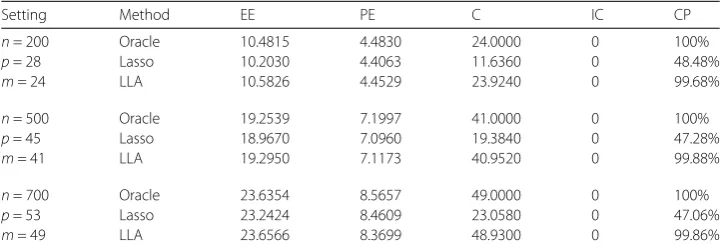
Table 3 Simulation results for LAD loss function andε∼0.9N(0, 1) + 0.1N(0, 9)

Setting Method EE PE C IC CP

n= 200 Oracle 10.4815 4.4830 24.0000 0 100%

p= 28 Lasso 10.2030 4.4063 11.6360 0 48.48%

m= 24 LLA 10.5826 4.4529 23.9240 0 99.68%

n= 500 Oracle 19.2539 7.1997 41.0000 0 100%

p= 45 Lasso 18.9670 7.0960 19.3840 0 47.28%

m= 41 LLA 19.2950 7.1173 40.9520 0 99.88%

n= 700 Oracle 23.6354 8.5657 49.0000 0 100%

p= 53 Lasso 23.2424 8.4609 23.0580 0 47.06%

m= 49 LLA 23.6566 8.3699 48.9300 0 99.86%

is slightly higher than that of the case where the error term is a standardized normal dis-tribution. The reason is that when the error term is heavy tailed, it is more appropriate to choose LLA, but the accuracy of estimation and prediction is slightly worse than that of Lasso. When the sample size increases, the LLA and Oracle estimates perform equally well in the selection of important variables and the complexity of the model.

bet-Table 4 Simulation results for Huber loss function andε∼N(0, 1)

Setting Method EE PE C IC CP

n= 200 Oracle 10.8300 3.3696 24.0000 0 100%

p= 28 Lasso 9.6422 3.5569 20.0920 0 83.72%

m= 24 LLA 10.9088 3.3784 22.7200 0 94.67%

n= 500 Oracle 19.9141 5.4034 41.0000 0 100%

p= 45 Lasso 18.0691 5.6068 38.0300 0 92.76%

m= 41 LLA 19.8884 5.3937 40.5160 0 98.82%

n= 700 Oracle 24.3265 6.3761 49.0000 0 100%

p= 53 Lasso 22.4030 6.5988 46.2440 0 94.38%

m= 49 LLA 24.3596 6.3882 48.6620 0 99.31%

Table 5 Simulation results for Huber loss function andε∼t5

Setting Method EE PE C IC CP

n= 200 Oracle 10.5572 4.2666 24.0000 0 100%

p= 28 Lasso 9.2590 4.4065 18.4680 0.0020 76.95%

m= 24 LLA 10.6099 4.2429 22.8100 0 95.04%

n= 500 Oracle 19.4395 6.8118 41.0000 0 100%

p= 45 Lasso 17.4385 6.9993 36.2080 0 88.31%

m= 41 LLA 19.4471 6.8247 40.5440 0 98.89%

n= 700 Oracle 23.8089 8.0487 49.0000 0 100%

p= 53 Lasso 21.6534 8.2558 44.4980 0 90.81%

m= 49 LLA 23.8220 8.0807 48.6940 0 99.38%

Table 6 Simulation results for Huber loss function andε∼0.9N(0, 1) + 0.1N(0, 9)

Setting Method EE PE C IC CP

n= 200 Oracle 10.4829 4.4694 24.0000 0 100%

p= 28 Lasso 9.1630 4.6333 18.0680 0 75.28%

m= 24 LLA 10.5706 4.4827 22.7880 0 94.95%

n= 500 Oracle 19.2618 7.1860 41.0000 0 100%

p= 45 Lasso 17.3780 7.3190 35.3500 0 86.22%

m= 41 LLA 19.2962 7.2029 40.5900 0 99.00%

n= 700 Oracle 23.6356 8.5563 49.0000 0 100%

p= 53 Lasso 21.5202 8.7148 43.4420 0 88.66%

m= 49 LLA 23.6275 8.5822 48.7120 0 99.41%

ter than the Lasso method. The reason for this is that the real data has a mixed normal distribution with high probability.

5 Conclusion

Funding

The work was supported by the NSFC (71803001, 61703001), the NSF of Anhui Province (1708085MA17, 1508085QA13), the Key NSF of Education Bureau of Anhui Province (KJ2018A0437) and the Support Plan of Excellent Youth Talents in Colleges and Universities in Anhui Province (gxyq2017011).

Competing interests

The authors declare that they have no competing interests.

Authors’ contributions

All authors contributed equally to the writing of this paper. All authors read and approved the final manuscript.

Publisher’s Note

Springer Nature remains neutral with regard to jurisdictional claims in published maps and institutional affiliations.

Received: 16 March 2018 Accepted: 16 August 2018

References

1. Huber, P.: Robust estimation of a location parameter. Ann. Math. Stat.35, 73–101 (1964)

2. Huber, P.: Robust regression: asymptotics, conjectures and Monte Carlo. Ann. Stat.1, 799–821 (1973) 3. Huber, P.: Robust Statistics. Wiley, New York (1981)

4. Portnoy, S.: Asymptotic behavior of M-estimators of p regression parameters whenp2_{/nis large, I: consistency. Ann.}

Stat.12, 1298–1309 (1984)

5. Welsh, A.: On M-processes and M-estimation. Ann. Stat.17, 337–361 (1989)

6. Mammen, E.: Asymptotics with increasing dimension for robust regression with applicationsto the bootstrap. Ann. Stat.17, 382–400 (1989)

7. Bai, Z., Wu, Y.: Limiting behavior of M-estimators of regression coefficients in high dimensional linear models I. Scale-dependent case. J. Multivar. Anal.51, 211–239 (1994)

8. He, X., Shao, Q.: On parameters of increasing dimensions. J. Multivar. Anal.73, 120–135 (2000)

9. Li, G., Peng, H., Zhu, L.: Nonconcave penalized M-estimation with a diverging number of parameters. Stat. Sin.21, 391–419 (2011)

10. Zou, H., Li, R.: One-step sparse estimates in nonconcave penalized likelihood models. Ann. Stat.36, 1509–1566 (2008) 11. Bai, Z., Rao, C., Wu, Y.: M-estimation of multivariate linear regression parameters under a convex discrepancy function.

Stat. Sin.2, 237–254 (1992)

12. Wu, W.: M-estimation of linear models with dependent errors. Ann. Stat.35, 495–521 (2007)

13. Huang, J., Horowitz, J., Ma, S.: Asymptotic properties of bridge estimators in sparse high-dimensional regression models. Ann. Stat.36, 587–613 (2008)