A Parametric Model of Cervical Spine
Geometry and Posture
Final Report
UMTRI-2017-1
Matthew P. Reed
Monica L.H. Jones
Biosciences Group
University of Michigan Transportation Research Institute
A Parametric Model of Cervical Spine Geometry and Posture
Final Report
UMTRI-2017-1
by
Matthew P. Reed Monica L.H. Jones
University of Michigan Transportation Research Institute
REPORT DOCUMENTATION PAGE
OMB No. 0704-0188 Form Approved Public reporting burden for this collection of information is estimated to average 1 hour per response, including the time for reviewing instructions, searching existing data sources, gathering and maintaining the data needed, and completing and reviewing this collection of information. Send comments regarding this burden estimate or any other aspect of this collection of information, including suggestions for reducing this burden to Department of Defense, Washington Headquarters Services, Directorate for Information Operations and Reports (0704-0188), 1215 Jefferson Davis Highway, Suite 1204, Arlington, VA 22202-4302. Respondents should be aware that notwithstanding any other provision of law, no person shall be subject to any penalty for failing to comply with a collection of information if it does not display a currently valid OMB control number. PLEASE DO NOT RETURN YOUR FORM TO THE ABOVE ADDRESS.1. REPORT DATE (DD-MM-YYYY)
February 2017 2. REPORT TYPEFinal Report 3. DATES COVERED (From - To)
4. TITLE AND SUBTITLE 5a. CONTRACT NUMBER
W56HZV-04-2-0001 P00038
A Parametric Model of Cervical Spine Geometry and Posture 5b. GRANT NUMBER
5c. PROGRAM ELEMENT NUMBER
6. AUTHOR(S) 5d. PROJECT NUMBER
Reed, Matthew P. and Jones, Monica L.H. 5e. TASK NUMBER 5f. WORK UNIT NUMBER
7. PERFORMING ORGANIZATION NAME(S) AND ADDRESS(ES)
AND ADDRESS(ES)
8. PERFORMING ORGANIZATION REPORT
NUMBER
University of Michigan
Transportation Research Institute UMTRI-2017-1
9. SPONSORING / MONITORING AGENCY NAME(S) AND ADDRESS(ES) 10. SPONSOR/MONITOR’S ACRONYM(S)
US Army Natick Soldier Research, Development, and Engineering Center, Natick, MA
Prime: Johns Hopkins Applied Physics Laboratory 11. SPONSOR/MONITOR’S REPORT NUMBER(S)
Issued Upon Submission
12. DISTRIBUTION / AVAILABILITY STATEMENT
13. SUPPLEMENTARY NOTES
14. ABSTRACT
Computational models of the cervical spine are useful tools for research on the biomechanics of neck injury and the
evaluation of countermeasures. This report describes the development of a parametric model of cervical spine geometry that is intended to provide input to computational modeling. Two-dimensional landmark data describing the outlines of the bones of the cervical spine and important head landmarks were obtained from lateral radiographs of volunteers in a seated posture
taken in a previous study. After imputation and a scaling adjustment, principal component analysis was performed on neutral-posture landmark data from 140 men and women with a wide range of age and body size. The first principal component was primarily related to spine curvature, whereas the second was associated with overall size. A
regression analysis predicting principal component scores from subject covariates found significant effects of stature, age, and the ratio of sitting height to stature. Sex was not a significant predictor of principal component scores after accounting for overall body size. A three-dimensional bone shape prediction was created using bone geometry from 38 women extracted from CT studies. A principal component analysis performed on each bone level from C1 to C7 demonstrated that the dominant mode of variation was overall size for C2 but not for the other levels. A detailed examination of vertebra dimensions showed that length, width, and height of the vertebrae and the vertebral bodies at C3 through C7 were not correlated. Two methods for generating 3D geometry to match the 2D predictions were created. First, a method was developed to compute the optimal vector of principal component scores such that the side-view projection of landmarks on the 3D bone best matched the 2D targets. Second, a method based on least-squares alignment and uniform scaling was developed. The method based on principal component scores aligned to the landmarks in the 3D dataset with average root-mean-square (RMS) errors below 1 mm, and matched the mesh with average RMS errors less than 2 mm. When aligning to landmarks generate from the 2D model, RMS errors were less than 2 mm. The RMS errors for the scaling method were only slightly larger. Both the PCAR 2D model and the scaling method for generating 3D bone models were implemented in the Python language for use by other researchers.
15. SUBJECT TERMS
Anthropometry, Cervical Spine
16. SECURITY CLASSIFICATION OF: 17. LIMITATION
OF ABSTRACT 18. NUMBER OF PAGES 19a. NAME OF RESPONSIBLE PERSON M.P. Reed a. REPORT
TBD
b. ABSTRACT
TBD
c. THIS PAGE
TBD 43
19b. TELEPHONE NUMBER
(include area code)
ACKNOWLEDGMENTS
CONTENTS
ABSTRACT 6
INTRODUCTION 7
METHODS 8
RESULTS 22
DISCUSSION 36
REFERENCES 40
APPENDIX A. Mean Spine Geometry 42
ABSTRACT
Computational models of the cervical spine are useful tools for research on the
biomechanics of neck injury and the evaluation of countermeasures. This report describes the development of a parametric model of cervical spine geometry that is intended to provide input to computational modeling. Two-dimensional landmark data describing the outlines of the bones of the cervical spine and important head landmarks were obtained from lateral radiographs of volunteers in a seated posture taken in a previous study. After imputation and a scaling adjustment, principal component analysis was
performed on neutral-posture landmark data from 140 men and women with a wide range of age and body size. The first principal component was primarily related to spine curvature, whereas the second was associated with overall size.
A regression analysis predicting principal component scores from subject covariates found significant effects of stature, age, and the ratio of sitting height to stature. Sex was not a significant predictor of principal component scores after accounting for overall body size.
A three-dimensional bone shape prediction was created using bone geometry from 38 women extracted from CT studies. A principal component analysis performed on each bone level from C1 to C7 demonstrated that the dominant mode of variation was overall size for C2 but not for the other levels. A detailed examination of
vertebra dimensions showed that length, width, and height of the vertebrae and the vertebral bodies at C3 through C7 were not correlated.
Two methods for generating 3D geometry to match the 2D predictions were created. First, a method was developed to compute the optimal vector of principal
INTRODUCTION
The cervical spine provides a high level of mobility to the head but is vulnerable to injury due to both chronic and acute loading. Computational modeling of the cervical spine (c-spine) and neck has been useful in understanding the influence of both direct and inertial loading on the head and thorax on c-spine kinematics and tissue strains. However, most c-spine models have used geometry from midsize males, and most c-spine geometry data have been extracted from medical images obtained in supine postures rather than postures corresponding to the loading scenarios of interest.
The current work addresses the need for parametric models of c-spine geometry and posture for men and women with a wide range of body size in seated postures with an unsupported head. These postures are typical of people in vehicle
environments, including military ground vehicles and aircraft.
The model developed in this work is based on two data sources: (1) a large-scale study of c-spine geometry and posture conducted by UMTRI in the 1970s using lateral radiographs, and (2) c-spine bone geometry extracted by our collaborators at Johns Hopkins Applied Physics Laboratory (APL) using novel techniques developed for the current work (Drenkow et al. 2017).
The methods for 2D model creation are based in large part on previous work at UMTRI on modeling skeletal structures and whole-body surface shapes. A principal component analysis (PCA) was used to explore the principal modes of variation in the dataset. Linear regression was used to test the effects of subject covariates on the size and shape of the c-spine vertebra and to create a predictive model.
A methodology for mapping 3D bone geometry to 2D landmark configurations was adapted from a method previously developed for fitting whole-body shape models to low-resolution scan data. A second method using least-squares fitting to the landmark locations was also tested.
METHODS
Data Sources
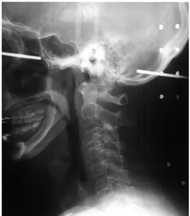
[image:8.595.163.432.261.567.2]The two-dimensional landmark data used to create the parametric geometry and posture model were obtained from Snyder et al. (1975). A total of 180 men and women with a wide range of age and body size were sat in a laboratory mockup with an unsupported head and horizontally directed vision. Lateral radiographs (Figure 1) were taken in the neutral posture and at maximum flexion and extension. In more recent work (Klinich et al. 2004), the original radiographs were digitized and a large number of landmark locations on the bones were manually extracted. These data have formed the basis for the development of new ways to represent cervical spine posture (Klinich et al. 2012).
Figure 1. Example of a lateral radiograph in the neutral posture from Snyder et al. (1975).
Imputation and Adjustment of Landmark Data
1. Missing landmarks in the flexed and extended postures were imputed by aligning the neutral-posture configuration using the available landmarks.
2. The landmarks for each bone in the three postures were aligned using generalized Procrustes, which performs a least-squares alignment.
3. The mean landmark configuration was computed.
4. The mean landmark configuration was aligned to the landmark data in each posture using a least-squares method. This aligned mean configuration was used for subsequent analysis.
Due to these steps, no data were missing and the shapes of the bones for each individual were invariant across postures.
Scaling the UMTRI 2D Data
During the process of developing the 3D model, a discrepancy was noted between the dimensions of the 2D model and those obtained from the APL 3D data. Further investigation was conducted to identify the source of the discrepancy. The 2D landmark locations obtained by digitizing the radiographs were originally scaled by reference to an array of beads oriented vertically in each image (see Figure 1). Snyder et al. (1975) data reports that these beads were “one inch” (i.e., 25.4 mm) apart and located on the “midsagittal plane”. The analysis by Klinich et al. (2004, 2007) assumed this scaling relationship. However, a closer examination of the images shows that in most cases the images of the beads overlap that of the head, indicating that the beads were placed adjacent to the head, and not in the
midsagittal plane. A detailed review of the study documentation did not reveal an alternative location for the beads. Fortunately, the detailed presentation of data in the Snyder report enabled the estimation of a correction factor.
Snyder et al. (1975) reported “segment lengths” based on the distances between “joint centers”, defined as the midpoints of the intervertebral spaces, using the tip of the dens as the upper margin of C2. The results were reported separately for men and women. Tables 1 and 2 list the segment lengths for men and women, along with the total, from Snyder et al. (1975). For comparison, comparable lengths were computed in the 2D landmark data, using the mean of the adjacent anterior and posterior vertebral body landmarks as an estimate of the “joint center.” Tables 1 and 2 list these along with the corresponding correction factor defined by the
relationship.
Table 1
Segment Lengths – Male (mm)
Snyder (in)* Snyder (mm) Original 2D Ratio
C2 1.509 38.32 47.4 0.808
C3 0.7054 17.92 22.5 0.796
C4 0.6895 17.51 21.8 0.803
C5 0.6715 17.06 21.1 0.808
C6 0.6670 16.94 20.8 0.815
C7 0.7215 18.33 19.3 0.950
Total 4.937 125.41 152.9 0.820
* Rounded to four digits
Table 2
Segment Lengths -- Female
Snyder (in)* Snyder (mm) Original 2D Ratio
C2 1.386 35.21 43.2 0.815
C3 0.6207 15.77 19.6 0.804
C4 0.6160 15.65 18.9 0.828
C5 0.6014 15.28 18.5 0.826
C6 0.6000 15.24 19.2 0.794
C7 0.6548 16.63 19.3 0.862
Total 4.478 113.7 138.7 0.820
* Rounded to four digits
Parametric 2D Spine Geometry Modeling
Some subjects from the Snyder sample were excluded due to problems with
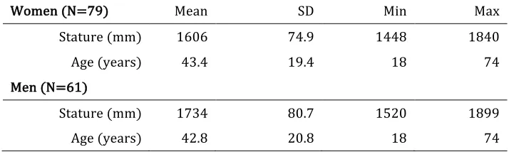
landmark availability. For example, in some flexed and extended scans, insufficient landmarks were in view to fit all of the vertebra segments and head. Out of the original 180 subjects, a total of 140 men and women with complete landmark sets following imputation were retained for analysis. Table 3 lists summary statistics for these subjects.
advantages of PCA for this application are that (1) a large percentage of the variance in the data can be expressed using a relatively small number of values, (2) the major modes of variance in spine geometry can be visualized, and (3) the subsequently developed regression models are independent on each principal component (PC).
Table 3
Summary Statistics for 2D Geometry Sample
Women (N=79) Mean SD Min Max
Stature (mm) 1606 74.9 1448 1840
Age (years) 43.4 19.4 18 74
Men (N=61)
Stature (mm) 1734 80.7 1520 1899
Age (years) 42.8 20.8 18 74
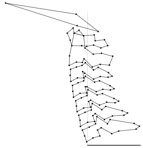
The coordinates of the spine landmarks in the neutral posture were first aligned to a T1 coordinate system with the origin at the anterior superior body landmark and the positive X axis passing through the posterior T1 spinous process landmark, as shown in Figure 2. The mean T1 angle with respect to global horizontal was 3.2 degrees (sd 7.3 degrees), indicating that the T1 spinous process landmark was on average slightly higher than the anterior-superior T1 body landmark. No significant relationships between body dimensions or age and T1 angle were found. The
coordinate data for the 122 landmarks were used. Table 4 describes the landmark naming convention. Table 5 lists the landmarks, which are depicted in
representative radiographs in Figures 3 and 4. The head landmarks are infraorbitale, tragion, and the anterior and posterior margins of the occipital condyles.
The landmark coordinates were collapsed into a single geometry vector of 244 elements and the PCA was performed on the covariance matrix. A regression analysis was then conducted using sex, stature, age, body mass index (weight in kg divided by the square of stature in meters), the ratio of sitting height to stature, and the interactions between sex and the other variables as potential predictors of principal component (PC) scores. The regression models were assessed with respect to the statistical significance of the predictors and the overall adjusted R2 values.
Figure 2. Illustration of landmarks (connected by lines) used in PCA. Horizontal line at the bottom of plot connects anterior-superior body and spinous process landmarks of T1 and defines the
coordinate system in which the neutral spine geometry was modeled.
Table 4
Abbreviations in Landmark Names
Abbreviation Definition
Ant Anterior
Pos Posterior
Sup Superior
Inf Inferior
Med Median
SpiPro Spinous Process Bod Body of Vertebra Den Dens (C2)
Tub Tubercle
C1C2 Apparent intersection of the outlines of C1 and C2
Arc Arch
Can Canal
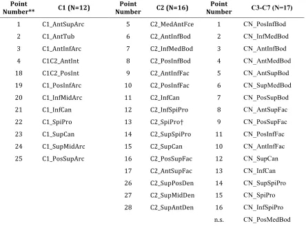
[image:12.595.130.488.442.692.2]Table 5
List of Landmarks* Used in PCA
Point
Number** C1 (N=12) Number Point C2 (N=16) Number Point C3-C7 (N=17)
1 C1_AntSupArc 5 C2_MedAntFce 1 CN_PosInfBod
2 C1_AntTub 6 C2_AntInfBod 2 CN_InfMedBod
3 C1_AntInfArc 7 C2_InfMedBod 3 CN_AntInfBod
4 C1C2_AntInt 8 C2_PosInfBod 4 CN_AntMedBod
18 C1C2_PosInt 9 C2_AntInfFac 5 CN_AntSupBod
19 C1_PosInfArc 10 C2_PosInfFac 6 CN_SupMedBod
20 C1_InfMidArc 11 C2_InfCan 7 CN_PosSupBod
21 C1_InfCan 12 C2_InfSpiPro 8 CN_AntSupFac
22 C1_SpiPro 13 C2_SpiPro† 9 CN_PosSupFac
23 C1_SupCan 14 C2_SupSpiPro 11 CN_PosInfFac
24 C1_SupMidArc 15 C2_SupCan 10 CN_AntInfFac
25 C1_PosSupArc 16 C2_PosSupFac 12 CN_SupCan
17 C2_AntSupFac 13 CN_InfCan
26 C2_SupPosDen 14 CN_SupSpiPro
27 C2_SupMidDen 15 CN_SpiPro
28 C2_SupAntDen 16 CN_InfSpiPro
n.s. CN_PosMedBod
* Abbreviations in landmark names are given in Table 4.
** See Figures 3 and 4.
Figure 3. Landmarks digitized on C1 and C2 (Klinich et al. 2004).
[image:14.595.85.513.405.674.2]Spine Articulation
[image:15.595.125.475.298.497.2]The three measurement postures provide an opportunity to characterize the spine motion patterns. Ranges of motion can be calculated for each segment based on the differences in orientation of the vertebra between flexed, neutral, and extended postures. Table 6 summarizes range of motion values by level as reported by Snyder et al. (1975). Note that C1 motion with respect to C2 was not quantified. The mean total range of head motion (ROM) with respect to T1 for all subjects in the Snyder dataset was 117 degrees (sd 24 degrees).
Table 6
Total Mean ROM by Motion Segment from Snyder et al. (1975)
Level ROM (degrees) Fraction of Head/T1
Head/C1 22.4 0.192
C1/C2 (not measured)
C2/C3 4.5 0.038
C3/C4 13.2 0.104
C4/C5 23.0 0.197
C5/C6 21.2 0.181
C6/C7 18.7 0.160
C7/T1 15.0 0.128
C2/T1 (sum of above) 94.6 0.809
Head/T1 117 1
With only three postures, it is not possible to characterize the distribution of spine motion for intermediate postures. As an approximation, a spine articulation method was used that distributes motion among the segments according to the fractions of total ROM at each level listed in Table 6. The articulation model is driven by the change from the neutral posture in head orientation relative to T1.
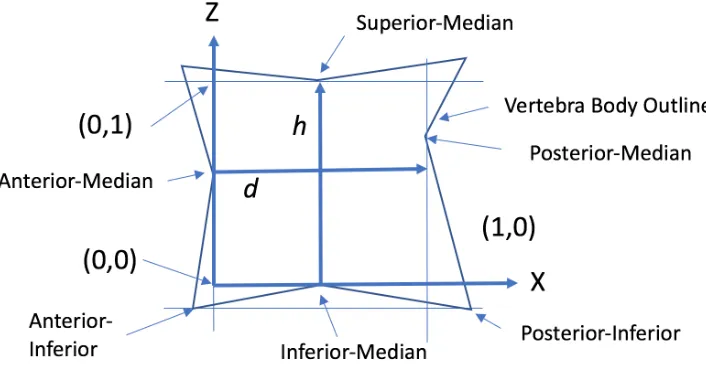
landmark. The vertical axis is established perpendicular to the horizontal axis such that it passes through the anterior median body landmark. The height (h) and depth (d) of the vertebral body are computed from the axes to the lines passing through the superior and posterior median body landmarks.
Table 7 lists the scaled-coordinate locations for each motion center. Figure 6 shows the motion centers on the mean neutral spine. The C7/T1 rotation center was not given by Amevo, and the T1 geometry is not complete in the current dataset. Consequently, the C7/T1 motion center location was estimated with respect to C7 (scaled Z coordinate is negative).
[image:16.595.92.520.530.677.2]Figure 5. Establishing a coordinate system equivalent to Amevo et al. (1991).
Table 7
C2 through C7 Motion Centers in Scaled* Coordinates from Amevo et al. (1991)
Moving Vertebra Vertebra Relative to Which Motion Center
is Estimated
X Coordinate (scaled) Z Coordinate (scaled)
C2 C3 0.27 0.36
C3 C4 0.32 0.52
C4 C5 0.36 0.60
C5 C6 0.39 0.78
C6 C7 0.44 0.95
C7† C7 0.50 -0.05
* Horizontal and vertical coordinates are scaled by the vertebral body depth and height, respectively; see Figure 5.
Figure 6. Motion centers (red circles) and intervertebral points (black circles).
Three-Dimensional Vertebra Model
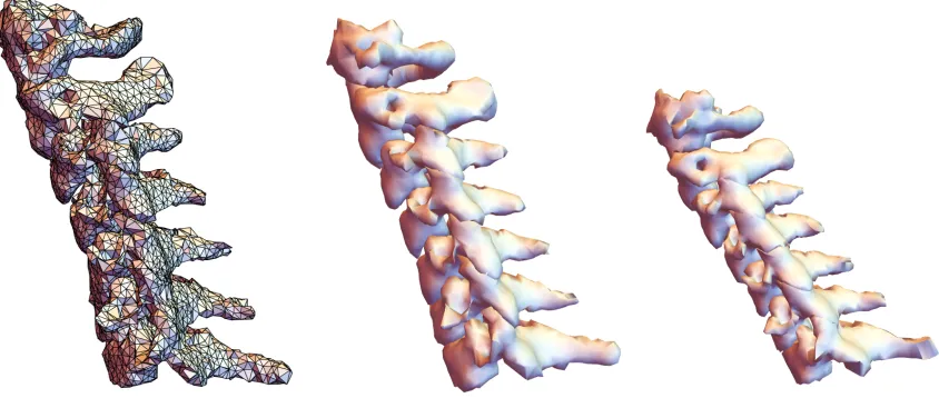
One goal of the project was to develop a method to predict three-dimensional bone shape as a function of the landmark data available in the 2D spine geometry model. Our collaborators at Johns Hopkins Applied Physics Laboratory (APL) developed a pipeline for automated extraction of c-spine bone geometry from CT studies. The methodology for bone extraction is covered in a separate report from APL. In brief, a finite-element mesh was fit to the CT density data using a semi-automated
procedure, so each bone is represented by a homologous set of surface node (mesh vertices).
Figure 7. Example spine meshes obtained from CT scans of supine patients. The image on the left shows the individual polygons. The other images are rendered using smooth shading.
Predicting 3D Vertebra Shape from 2D Landmarks: PC Method
The parametric 2D spine model predicts the size and positioning of vertebra but does not predict the full 3D geometry of the bones. To address this issue, a method was developed to link the 3D vertebra geometry to the 2D landmark model to obtain a parametric 3D spine model. The advantages of linking to the 2D model are (1) inclusion of the effects of the stature covariate on bone size and position and (2) representation of the neck posture with an unsupported head.
The method for predicting 3D geometry was as follows:
1. For each bone level:
a. Align all bones using generalized Procrustes alignment and restore scale. b. Compute the mean bone.
c. Manually identify vertices on the bone corresponding to the 2D landmarks. (This was performed by one individual.)
d. Perform a PCA on the bone meshes
2. Generate 2D spine geometry prediction for all bones from statistical model as described above.
3. For each bone, compute the 3D bone shape that best fits the selected landmark locations.
a. Compute the optimal (least squares) alignment of the 2D data to the 3D model using the landmarks listed in Table 4.
c. Align the resulting 3D bone to the 2D spine in position.
An iterative process was used to fit the 3D PCA model for each bone to the selected 2D landmarks. At each iteration, the algorithm took the following steps:
1. Align the 2D and 3D landmarks in the XZ plane using a least-squares fit. 2. Compute the optimal set of values for PC to align the XZ projection of the 3D
landmarks with the 2D landmarks (see below for details of this calculation). 3. If iteration has not converged, return to step 1.
4. Apply this vector of PC scores to obtain the full set of surface coordinates for the vertebra.
The optimal vector of PC scores is calculated by exploiting the linear relationship between PC scores and landmark coordinates. Specifically, the individual values in the PC vector represent the rate of change of node coordinates with a unit change in each PC score. Hence, extracting those columns from the PC matrix yields a
sensitivity matrix S.
UpdatedPCScores = CurrentPCScores + (CurrentCoordinates-TargetCoordinates).pinv(S)
where pinv is the Moore-Penrose pseudoinverse. This approach calculates the minimum-norm vector of PC scores that will match the coordinates.
To improve the quality of fitting, a new method was developed to limited the range of the calculated PC scores within a range defined by a combination of the range of values in the data and the relative fraction of variance accounted for by the PC. First, a PC weight is assigned based on the relative fraction of variance accounted for in the PCA, with the first PC assigned a value of 1. Second, this weight wi is used to
define a bound for each PC’s scores as ± wi p s where s is the standard deviation of
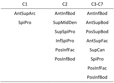
Table 8
Landmarks Used for 2D->3D Mapping
C1 C2 C3-C7
AntSupArc AntInfBod AntInfBod SpiPro SupMidDen AntSupBod
SupSpiPro PosSupBod InfSpiPro AntSupFac PosInfFac SupCan PosInfBod SpiPro
PosInfFac PosInfBod
Predicting 3D Vertebra Shape from 2D Landmarks: Scaling Method
The PC-based method provides a good alignment of the 3D landmarks to the 2D targets, but the bone shapes can become somewhat distorted. For some
applications, a smoother bone shape with slightly less accurate fitting to the landmark locations might be preferred. Consequently, an alternative method was developed that is computationally simpler and produces smoother bone shapes. The method scales and rotates the mean bone shape to obtain the best (least-squares) alignment to the target landmark locations.
1. Center the target and mean landmark locations by subtracting the respective means.
2. Compute the centroid size (defined as the square root of the sum of squared distances of each point from the origin) and divide the centered coordinates by their respective scales to obtain unscaled landmarks for both target and mean shape. For a matrix P of points pi = {xi, zi} the centroid size S is
S (mm) = tr(P. P T)1/2
where PT indicates the transpose and tr is the trace of the matrix (sum of
diagonal elements).
3. Compute the optimal (least-squares) side-view rotation to align the unscaled, centered landmarks from the mean shape to the unscaled, centered target landmarks. The method uses the singular value decomposition (SVD). For centered, unscaled P1 and P2, the matrix R to rotate P2 into P1 is given by
R = V.UT
4. For each vertex in the mean bone mesh,
a. subtract the mean of the mean mesh landmark locations b. scale by the ratio (target centroid size) / (mean centroid size) c. apply the rotation R around the Y axis
d. translate to the target mean
RESULTS
Parametric 2D Spine Geometry Model in Neutral Seated Posture
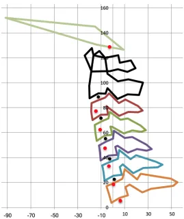
The mean 2D spine shape is tabulated in Appendix A. The first 6 PCs accounted for 97% of the variance, as shown in Figure 8. Figure 9 illustrates the first 6 PCs by manipulating the PC by ±3 standard deviations of the associated PC scores while holding the other scores at zero. Somewhat surprisingly, the first PC (65% of variance) is related to posture rather than body size. This demonstrates that the “neutral” neck posture associated with this task condition (seated with self-supported head with forward-oriented vision) is associated with a wide range of spine flexion. The second PC (27%) shows the overall size effect typically seen in PCA of biological structures, but also demonstrates an association between
[image:22.595.88.511.307.511.2]curvature and overall size. The third PC (3%) illustrates variance spine curvature independent of overall spine angle. The remaining PCs account for a total of 5% of variance and each individually less than 1%.
Figure 9. Illustration of PC effects by overlaying mean and geometry obtained by manipulating each PC by ±3 standard deviations of the associated PC scores. Neutral posture is shown in green. Percentage of total variance for PCs 1 through 6: 64.9, 26.9, 3.1, 0.8, 0.7, 0.6
The regression analyses were examined for the first six principal components. In no case was sex or the interaction between sex and another predictor significant in models containing stature. That is, after accounting for overall body size, sex did not have significant effects. Age and the ratio of sitting height to stature (typical value 0.52) were also significant for some PCs. Table 9 shows the significance levels for these predictors along with the adjusted R2 values for the models. Stature was
Table 9
Significance Test Results in Regression Models Predicting Principal Component (PC) Scores
PC Stature Age Sitting
Height/Stature R2adj Fraction of Variance from PCA
1 *** (+) *** (+) ** (+) 0.24 0.649
2 *** (-) ** (-) 0.52 0.269
3 * (+) 0.02 0.031
4 *** (-) 0.13 0.008
5 n.s. 0.007
6 *** (+) 0.27 0.006
* p<0.05; ** p<0.01; *** p<0.001
The actual geometric effects of the predictors over the ranges of interest are more important than the significance tests. To account for trends that do not reach statistical significance, all three predictors were included for all PCs in subsequent analyses. Figure 10 shows the effects of the stature from 1525 to 1870 mm (5th%ile
female to 95th%ile male in ANSUR II (Gordon et al. 2015), 0.500 to 0.546 (5th to
95th%ile for men and women in ANSUR II), and age 20 to 80 years.
Stature: 1525 to 1870 mm SH/S: 0.50 to 0.55 Age: 20 to 80 years
Figure 10. Illustration of participant covariate effects in neutral posture with the other variables held at mean values (1660 mm, 0.52, 44 years).
[image:24.595.82.454.403.574.2]samples matched on sitting height (17 males, 11 females) and head circumference (9 males, 18 females). Dimensions were extracted from CT reconstructions. Female dimensions were generally slightly smaller, although the differences were typically less than 10%.
Given these matched-sample findings, the reasons that the current modeling did not show sex effects after accounting for overall body size and age are not clear.
Figure 11 shows the result of including sex and interactions between sex, stature, SH/S, and age for all PCs. A small effect of sex is observed, with the predicted geometry being slightly smaller for women. For example, the A-P length of the C7 vertebra is 5% smaller in the predicted female geometry than in the male geometry. Comparing with the population effects in Figure 10, this analysis demonstrates that overall body size (stature and SH/S) have larger effects than sex across the
[image:25.595.210.391.364.596.2]population; that is, most of the differences in vertebra geometry in this data set are attributable to body size rather than sex. The reason for the sex-related spine-length difference in a model that accounts for stature and erect sitting height is unclear. Vadavada et al. (2008) found that a skeletal measure of neck length (vertical distance from C7 spinous process to tragion) was about 5% smaller in a group of women compared to a group of men matched on stature and external neck length, a difference that is consistent with Figure 11.
Figure 11. Effect of sex on spine geometry (male=black, female=red), including interactions with stature, SH/S, and age (stature = 1660 mm, SH/S = 0.52, age = 44 yrs).
Model Articulation
postures do not necessarily represent the kinematics of any individual, but at the extremes the model will accurately capture typical ranges of motion.
Midsize Male
Midsize Female
[image:26.595.80.515.115.420.2]-60˚ 0˚ 40˚
Figure 12. Illustration of spine articulation for change in head angle relative to T1 of -60, 0, and 40 degrees relative to neutral posture.
Covariance of Bone Dimensions
The 3D data provided an opportunity to examine the extent to which bone
dimensions are correlated at each vertebral level. Table 10 lists a set of dimensions extracted from each of the bones in the 38 c-spines obtained from CT. The
Table 10
Vertebral Dimensions Extracted from 3D Bone Meshes
Dimension Definition
Vertebra Length Maximum anterior-posterior dimension
Vertebra Width Maximum medial-lateral dimension
Vertebra Height Maximum vertical dimension
Vertebra Body Length Distance between anterior-inferior and posterior-inferior body landmarks Vertebra Body Width Distance between median-inferior left and
median-inferior right body landmarks
[image:27.595.86.509.383.660.2]Vertebra Body Height Distance between inferior and anterior-superior body landmarks.
Figures 13 and 14 shows cross plots of vertebra length and width and vertebral body length and width. For both pairs of dimensions, no relationships are observed, indicating that the lateral dimensions of the vertebrae are uncorrelated with the lengths (A-P dimensions) in this dataset.
Vertebra Width (mm)
Vertebra Length (mm)
Vertebra Body Width (mm)
[image:28.595.94.507.90.355.2]Vertebra Body Length (mm)
Figure 14. Vertebra body length (vertical axis) versus vertebra body width (horizontal axis) for bone meshes from 38 women (mm). Note differing scales in subplots.
Principal Component Analysis of 3D Bone Shapes
PC 1
PC2
PC3
[image:29.595.138.457.79.513.2]Front View Side View
PC 1
PC 2
PC 3
[image:30.595.81.497.78.517.2]Front View Side View
Figure 16. Effects of the first 3 principal components for C4. Overlays show ±3 SD (green and blue) on each of the first 3 components while holding other components at zero.
Results of Fitting 3D Models to 2D Geometry: PC Method
Figure 17 shows the results of fitting the 3D PCA models to the 2D model output for a midsize-female c-spine in several postures. To assess the accuracy of the
discrepancy observed across subjects was under 3 mm. For the mesh, the mean (across subjects) of the RMS error was less than 2 mm for all bones. The maximum discrepancy was largest for C1, at 3.65 mm, but the maximum RMS fitting error for the other bones was less than 2 mm.
Table 11
Fitting Errors* for Landmarks and Mesh: PCA Method (mm)
Bone Landmarks Mesh
Mean Minimum Maximum Mean Minimum Maximum
C1 0.28 0.00 0.93 1.90 1.17 3.65
C2 0.56 0.02 2.66 1.13 0.79 1.80
C3 0.34 0.02 2.01 0.93 0.62 1.33
C4 0.34 0.01 1.44 1.00 0.72 1.38
C5 0.45 0.03 2.93 0.98 0.72 1.33
C6 0.36 0.02 1.87 1.02 0.72 1.40
C7 0.46 0.02 2.64 1.25 0.76 1.73
* Root mean square error across 38 subjects (all of the spines used to generate the PC models).
The fitting performance was also assessed by evaluating how closely the fitted landmark locations matched the targets for spine profiles generated from the 2D model. Table 12 shows mean, minimum, and maximum RMS errors in coordinate values for a set of spines generated from the 2D model using statures from 1500 mm to 1750 mm in increments of 50 mm (approximately 5th-percentile female to
95th-percentile female). The RMS errors are somewhat larger than those observed in
the CT dataset, likely due to small differences in the placement of the landmarks relative to the bone. Nonetheless, the mean RMS errors are less than 1.5 mm across the 7 bones with maximum RMS errors less than 2 mm.
Table 12
Fitting Errors* for Landmarks for 6 Spine Profiles Generated from 2D: PC Method (mm)
Bone Landmarks
Mean Minimum Maximum
C1 0.33 0.03 0.82
C2 1.32 1.18 1.49
C3 0.99 0.66 1.32
C4 1.20 0.72 1.59
C5 0.96 0.74 1.10
C6 1.39 0.80 1.84
C7 1.30 1.21 1.38
[image:32.595.173.422.517.666.2]Results of Fitting 3D Models to 2D Geometry: Scaling Method
Table 13 presents the mean, minimum, and maximum RMS errors observed when applying the scaling method to the 3D bone meshes. As expected, both the landmark and mesh errors are larger than those obtained with the PC method, but the mean RMS landmark errors are below 1 mm and the mean RMS mesh errors are 2 mm or less.
[image:33.595.76.521.306.459.2]Table 14 shows the RMS errors in coordinate values for the same set of 2D spine profiles used for Table 12. Comparing to Table 12, the RMS errors are similar to those obtained using the PC method. This suggests that the PC method is not producing substantially better fit than the simpler scaling model to the landmark predictions from the 2D model.
Table 13
Fitting Errors* for Landmarks and Mesh: Scaling Method (mm)
Bone Landmarks Mesh
Mean Minimum Maximum Mean Minimum Maximum
C1 0.00** 0.00** 0.00** 2.01 1.07 3.57
C2 0.79 0.06 2.26 1.22 0.93 1.77
C3 0.69 0.02 2.66 1.08 0.79 1.95
C4 0.69 0.00 2.50 1.15 0.88 1.56
C5 0.82 0.05 3.68 1.18 0.82 2.12
C6 0.83 0.04 2.99 1.27 0.90 2.18
C7 0.94 0.07 3.96 1.50 0.89 2.65
* Root mean square error across 38 subjects.
Table 14
Fitting Errors* for Landmarks for 6 Spine Profiles Generated from 2D: Scaling Method (mm)
Bone Landmarks
Mean Minimum Maximum
C1 0.00** 0.00** 0.00**
C2 0.82 0.71 0.99
C3 1.19 1.15 1.24
C4 1.30 1.28 1.33
C5 1.12 1.09 1.18
C6 1.56 1.40 1.73
C7 1.17 1.08 1.29
* Root mean square error across 6 spine profiles generated from the 2D model. ** Due to the method, the landmark errors for C1, which uses only 2 landmarks for alignment, will always be zero.
Python Implementation of 2D Model
To facilitate use of the parametric spine geometry model, a version of the model was implemented in version 3.5 of the Python language (http://python.org/). The
Python version includes sex, stature, SH/S, age, and the head angle relative to neutral as inputs. Figure 18 shows a flow chart of the code, which is designed to be executed in a command-line environment. Appendix B contains a user guide for the software. Each time it is executed, the software loads the PC vectors, mean
Figure 18. Functional flow of Python implementation of 2D model.
Python Implementation of 3D Model
DISCUSSION
Two-Dimensional Model
The PCA of 2D landmark locations provided a clear demonstration that “neutral” spine posture is highly variable. Klinich et al. (2012) previously showed this using a spline to quantify curvature, but the current analysis demonstrates that posture dominates overall size in its contribution to the variance in landmark locations across a diverse subject pool. An important conclusion is that modeling aimed at assessing injury risk across a population should focus on posture variability at least as much as geometric variability.
The 2D cervical spine geometry model developed in this work provided an
opportunity to test hypotheses about the relationships between overall body size and neck geometry. The primary modes of variation in the spine, quantified by the principal components of the landmark coordinates, did not show significant variation by sex after taking into account overall body size using stature and the ratio of sitting height to stature. Body weight, quantified by body mass index, also did not have significant effects. Age had a small effect including a slightly more extended neck posture with age. An alternative model formulation that included sex predicted a slightly smaller spine for women, after taking into account stature, sitting height, and age, but the effect of sex and the associated interactions were not statistically significant for the first six principal components.
This 2D dataset used in this study is unusual in being obtained from a relatively large, anthropometrically diverse population in a seated posture with a self-supported head. Other 2D data are available, for example the large number of radiographs gathered in the Fels study (Roche 1992), some of which were obtained with a self-supported head. However, the greatest potential for improving the current work is through a larger collection of 3D data obtained from medical CT scans.
Nonetheless, the 2D model has several purposes not yet superseded by other
available tools. First, the simple formulation provides an easy way for developers of FE models to scale their cervical geometry accurately to represent individuals with a wide range of body size. For this purpose, the tool augments previous studies that have published distributions of bone dimensions. Importantly, the construction of the model ensures that the set of landmarks generated are internally consistent across a wide range of body size.
Second, and most importantly, the model generates the mean neutral spine
quantified the trends in head and thorax orientation with changes in seat back angle (e.g., Reed and Ebert 2013; Park et al. 2016); these may be used to adjust the
predicted postures. Another limitation for modeling applications is that the data do not take into account the effects of head-supported mass on posture.
A simple articulation model was implemented based on previously published segment rotation centers. Initially, the flexed and extended posture data were examined to determine if the motion centers could be calculated reliably. The results, however, were found to be highly variable and ultimately were discarded in favor of the literature values.
The utility of the articulation model is somewhat limited because the motion distribution is constant, which is not a realistic assumption at the limits of
movement. The articulation will be most useful for making small changes to account for different seating configurations, such as more-upright or more-reclined seating postures. Nonetheless, given the wide range of spine curvatures in “neutral”
postures, any discrepancies in spine curvatures obtained by this method will be small compared with the population variance. Importantly, this articulation model should not be taken to be representative of actual human movement.
Three-Dimensional Bone Shape Modeling
The analysis of bone shapes extracted from CT showed several surprising findings. First, the primary mode of variation for C3-C7 was not overall size, but rather a more complex relationship between size and shape. Second, consistent with that finding but more directly relevant for modeling, the overall length, width, and height of the bones were essentially uncorrelated. The same was true of the vertebral body, where no important scaling relationships were observed. This finding is limited by the relatively small and homogeneous sample (spines from 38 women), but even with that caveat the data strongly suggest that the major dimensions of the spine at the level of individual bones are not highly correlated.
For comparison, the 2D model shows a general scaling of the whole spine and the individual vertebra with overall body size (increased stature or sitting height). The 3D analysis suggests that the lateral dimensions likely are only weakly correlated with the overall size, at least for women. This somewhat surprising finding should be confirmed with a larger and more diverse sample. Nonetheless, it is consistent with the finding from the 2D landmark analysis of considerable idiosyncrasy in spine shape across individuals.
The method was developed under the assumption that a substantial amount of the lateral size and shape of the bones would be predictable from the 2D profile. In fact, as noted above, lateral dimensions are essentially uncorrelated with profile
dimensions in this 3D dataset. Consequently, the lateral dimensions of 3D spines generated by this method are similar across a range of neck lengths.
The 2D-to-3D mapping method generates a 3D model that closely corresponds to the predictions of the 2D model, but given the findings regarding bone shape variability, some simpler scaling methods might work similarly well. For example, the mean bone shape could be scaled in 3 dimensions to match the target vertebra size and aligned to the 2D predictions.
Alternative 3D Model Generation Methods
With a larger dataset, a number of alternative methods of generating a parametric 3D neck model are available.
1. A PCAR model of the whole spine can be created using subject covariates, such as sex, stature, and sitting height as predictors. However, sitting height is not
commonly available in patient database from which CT scans are extracted.
2. The c-spine length can be used as a size variable to predict the 3D shape, where the length is generated from the 2D model.
3. Because the data show that c-spine width is unrelated to height and depth, a geometric model of the c-spine can be scaled in side view using simple relationships based on the 2D model. For example, the vertebral height and anterior-posterior length could be used to perform affine scaling. This should produce results similar to the least-squares scaling method developed in the current work.
A central challenge in any landmark-based morphing method is finding truly homologous points. The larger landmark errors associated with fitting the 3D PCA model to 2D model outputs, compared with fitting to homologous points from the 3D dataset, indicates that the landmarks identified on the 3D model are not completely homologous. However, the differences are generally less than a millimeter, suggesting that only small improvements would be realized.
Limitations and Future Work
The accuracy of the 2D model is limited by the challenges in accurately and
consistently locating landmarks on the radiographs. Issues relating to this manual digitization process are discussed in Klinich et al. (2004) and in the original Snyder et al. (1975) report.
assumed to be appropriate for all subjects. The resulting model prediction using mean female anthropometry was similar in size to the mean 3D spine size, but it is possible that variable scaling factors were used in the original Snyder dataset. These would only affect the current analysis if the true scaling was correlated with one or more of the covariates. However, no indication of that is evident in either the Snyder et al. documentation or the data analysis.
The articulation method provides a reasonable way of adjusting postures around the neutral posture, and produces reasonable estimates at the extremes, due to the use of full flexion/extension range-of-motion to define the distribution of motion. However, the kinematics should not be taken to be representative of the average spine motion between postures for any individual.
The 3D analysis was based on relatively few subjects (38 women). A larger dataset would have provided more confidence in the outcome of the PCA on bone shapes and may have improved the performance of the PC-based fitting method. However, the scaling method, which uses only the average bone shape, would not be improved by the addition of more data.
REFERENCES
Amevo, B., Worth, D., and Bogduk, N. (1991). Instantaneous axes of rotation of the typical cervical motion segments: a study in normal volunteers. Clinical Biomechanics, 6:111-117.
Drenkow, N., Pyles, C., Kuo, N., Harrigan, T., Thawait, G., Fritz, J., Carneal, C. (2017).
Improved Head-Neck Finite Element Model for Dynamic Head Impact Simulation.
Technical Report. Johns Hopkins University Applied Physics Laboratory.
Li, Z., Park, B-K, Liu, W., Zhang, J., Reed, M.P., Rupp, J.D., Hoff, C.N., and Hu, J. (2015). A statistical skull geometry model for children 0-3 years old. PLOS One, 10(5). 10.1371/journal.pone.0127322
Klein, K.F., Hu, J., Reed, M.P., Hoff, C.N., and Rupp, J.D. (2015). Development and validation of statistical models of femur geometry for use with parametric finite element models. Annals of Biomedical Engineering, 43(10): 2503-2514. 10.1007/s10439-015-1307-6
Park, B-K and Reed, M.P. (2015). Parametric body shape model of standing children ages 3 to 11 years. Ergonomics, 58(10):1714-1725. 10.1080/00140139.2015.1033480 Klinich, K.D., Ebert, S.M., Van Ee, C.A., Flannagan, C.A., Prasad, M., Reed, M.P., and Schneider, L.W. (2004). Cervical spine geometry in the automotive seated posture: variations with age, stature, and gender. Stapp Car Crash Journal, 48:301-330. Klinich, K.D., Ebert, S.M., Reed, M.P.(2012). Quantifying cervical spine curvature using Bézier splines. Journal of Biomechanical Engineering, 11(4): 114503-114508. 10.1115/1.4007749
Gordon, C.C., Blackwell, C.L., Bradtmiller, B., Parham, J.L., Barrientos, P., Paquette, S.P., Corner, B.D., Carson, J.M., Venezia, J.Z., Rockwell, B.M., Mucher, M., and
Kristensen, S. (2015). 2012 Anthropometric Survey of U.S. Army Personnel: Methods and Summary Statistics. Technical Report NATICK/TR-15/007. U.S. Army Natick Soldier Research, Development and Engineering Center Natick, Massachusetts.
Park, J., Ebert, S.M., Reed, M.P., and Hallman, J.J. (2016). A statistical model including age to predict passenger postures in the rear seats of automobiles. Ergonomics, 59(6): 796-805, 10.1080/00140139.2015.1088076
Reed, M.P. and Ebert, S.M. (2013). The Seated Soldier Study: Posture and Body Shape in Vehicle Seats. Technical Report 2013-13. University of Michigan Transportation Research Institute, Ann Arbor, MI.
Snyder, R. G., Chaffin, D. B., and Foust, D. R. (1975). Bioengineering study of basic physical measurements related to susceptibility to cervical
hyperextension-hyperflexion injury. Final report UM-HSRI-BI-75-6, University of Michigan Transportation Research Institute, Ann Arbor, MI.
Stemper, B.D., Derosia, J.J., Yoganandan, N., Pintar, F.A., Shender, B.S., and Pasko, G.R. (2009) Gender dependent cervical spine anatomical differences in size-matched volunteers. Biomed Sci Instrum, 45:149-154.
Vasavada, A.N., Danarajb , J., and Siegmund, G.P. (2008). Head and neck
APPENDIX A
Mean 2D Spine Landmark Configuration (mm)
Abbreviations:
Ant Anterior
Pos Posterior
Sup Superior
Inf Inferior
Med Median
SpiPro Spinous Process Bod Body of Vertebra Den Dens (C2)
Tub Tubercle
C1C2 Apparent intersection of the outlines of C1 and C2
Arc Arch
Can Canal
Fac Facet
The origin is the anterior-superior body landmark on T1 (T1_ AntSupBod). The X axis is positive from T1_ AntSupBod to the T1 spinous process landmark (T1_SpiPro)
Landmark X Z
C2_SupAntDen -14.1 117.2 C1_AntSupArc -15.1 122.6
C1_AntTub -21.2 117.4
C1_AntInfArc -18.2 110.2
C1C2_AntInt -16.5 104.3
C1C2_PosInt -6.2 104.0
C1C2_PosInt -6.2 104.0
C1_PosInfArc -1.0 103.6
C1_InfMidArc 6.2 104.8
C1_InfCan 13.9 101.9
C1_SpiPro 21.0 104.3
C1_SupCan 17.5 110.4
C1_SupMidArc 7.9 109.2
C2_SupAntDen -14.1 117.2
C2_MedAntFac -18.9 93.5
C2_AntInfBod -19.0 83.5
C2_InfMedBod -11.8 87.0
C2_PosInfBod -5.6 86.6
C2_AntInfFac -3.6 90.5
C2_PosInfFac 4.9 81.9
C2_InfCan 13.1 84.7
C2_InfSpiPro 22.7 83.7
C2_InfSpiPro 22.7 83.7
C2_SupSpiPro 26.3 93.0
C2_SupCan 14.5 96.2
C2_PosSupFac 5.8 95.3
C2_AntSupFac -2.8 101.7
C2_SupPosDen -4.1 114.6
C2_SupPosDen -4.1 114.6
C2_SupMidDen -8.9 120.2
C2_SupAntDen -14.1 117.2
C3_AntInfBod -17.5 66.7
C3_AntMedBod -18.1 73.1
C3_AntSupBod -17.6 79.5
C3_SupMedBod -11.6 81.8
C3_PosSupBod -5.9 83.5
C3_AntSupFac -2.2 86.3
C3_PosSupFac 6.3 78.6
C3_SupCan 11.2 81.4
C3_SupSpiPro 21.6 76.1
C3_SpiPro 25.4 72.2
C3_InfSpiPro 21.5 71.1
C3_InfCan 13.1 71.9
C3_PosInfFac 6.2 69.1
C3_AntInfFac -2.9 75.5
C3_PosMedBod -5.0 77.0
C3_PosInfBod -4.0 70.4
C3_InfMedBod -10.7 70.4
C4_AntInfBod -14.6 50.4
C4_AntMedBod -15.3 56.5
C4_AntSupBod -15.8 62.6
C4_SupMedBod -9.8 65.2
C4_AntSupFac -2.3 72.3
C4_PosSupFac 7.1 66.0
C4_SupCan 12.3 67.5
C4_SupSpiPro 23.4 62.4
C4_SpiPro 27.6 59.0
C4_InfSpiPro 23.8 57.8
C4_InfCan 15.7 58.6
C4_PosInfFac 9.0 56.0
C4_AntInfFac -0.7 61.2
C4_PosMedBod -2.5 61.2
C4_PosInfBod -1.0 54.9
C4_InfMedBod -7.8 54.4
C5_AntInfBod -11.1 35.1
C5_AntMedBod -11.5 41.1
C5_AntSupBod -12.4 46.6
C5_SupMedBod -6.5 49.6
C5_PosSupBod -0.6 52.0
C5_AntSupFac 0.6 58.2
C5_PosSupFac 9.9 52.5
C5_SupCan 15.5 54.0
C5_SupSpiPro 27.6 49.0
C5_SpiPro 32.4 46.2
C5_InfSpiPro 28.6 44.4
C5_InfCan 20.0 44.9
C5_PosInfFac 12.6 42.0
C5_AntInfFac 3.2 47.1
C5_PosMedBod 1.3 45.9
C5_PosInfBod 3.0 39.9
C5_InfMedBod -4.1 39.1
C6_AntInfBod -7.5 19.8
C6_AntMedBod -8.0 26.0
C6_AntSupBod -9.3 31.5
C6_SupMedBod -2.6 34.4
C6_PosSupBod 3.7 37.0
C6_AntSupFac 4.8 43.9
C6_PosSupFac 14.9 37.3
C6_SupCan 19.0 40.6
C6_SupSpiPro 36.2 36.0
C6_InfCan 25.7 30.7
C6_PosInfFac 17.5 27.0
C6_AntInfFac 8.1 33.2
C6_PosMedBod 5.5 31.0
C6_PosInfBod 7.2 24.9
C6_InfMedBod -0.1 24.0
C7_AntInfBod -1.1 3.6
C7_AntMedBod -3.0 9.8
C7_AntSupBod -5.4 15.8
C7_SupMedBod 1.8 19.1
C7_PosSupBod 8.2 22.3
C7_AntSupFac 9.8 29.9
C7_PosSupFac 20.6 22.6
C7_SupCan 23.4 26.8
C7_SupSpiPro 48.4 22.9
C7_SpiPro 53.9 19.9
C7_InfSpiPro 50.5 16.8
C7_InfCan 32.5 14.9
C7_PosInfFac 25.3 12.3
C7_AntInfFac 14.2 18.3
C7_PosMedBod 10.5 16.0
C7_PosInfBod 12.8 9.7
C7_InfMedBod 5.6 7.7
Tragion -11.9 137.1
Infraorbitale -85.6 148.7
AntOccCon -10.9 125.0
APPENDIX B
User Guide to Software Implementation
UMTRI Parametric C-Spine Model
Software for generating 2D and 3D cervical spine bone geometry as a function of anthropometry and posture.
Author: [email protected]
Revision Date: 2017-02-25
***********
Python version 3.x is required; tested with Python version 3.5.
The numpy library is required.
***********
>>> from CSpine2DPCAR import *
# anthro.FEMALE and anthro.MALE are defined as 1 and -1, respectively
# shs = sitting height / stature
>>> target_anthro = anthro(anthro.FEMALE, stature=1650, age=45, shs=0.52)
>>> pcar = PCARSpine2D()
>>> pcar.predict(target_anthro, delta_head_angle=-30)
# delta head angle from neutral in degrees; negative is flexion
The predict() methods generates a spine using the PCAR model, articulates the model according to the delta_head_angle, then writes the model to a file
"SpineOut.tsv" that contains named points.
The PCARSpine2D.predict() method can also be called with keyword arguments:
>>> pcar.predict(sex=anthro.FEMALE, stature=1750, age=45, delta_head_angle=20)
or with a list of anthro:
>>> pcar.predict(anthro=[1, 1750, 0.52, 45], delta_head_angle=20) # sex: -1=male, 1=male
The module can also be run from the command prompt with the anthro and posture as command-line arguments
$ python CSpine2DPCAR.py 1 1650 0.52 20 0
Note all five arguments (sex, stature, shs, age, and delta head angle) must be supplied. If none is supplied, a midsize female spine is generated in the neutral posture.
A location parameter can be added to the predict() call to translate and rotate the model. Using the argument location='C7' (or other level up to C2) will place the anterior-inferior margin of the body at the origin and align the inferior surface of the body with the global x axis. Alternatively, enter a location and angle, e.g., [[40, 40], 30] will translate the model by [40, 40] and rotate 30 degrees clockwise. The segment positions and orientations are written at the end of the landmark file.
Running CSpine2DPCAR from the command line (executing the module) will automatically run CSpine3DFitting on the result.
***********
CSpine3DFitting.py
Usage:
>>> from CSpine3DFitting import *
>>> bm = BoneMapper()
The file SpineOut.tsv residing in the output directory is read. The 3D geometry in the data directory is mapped to the 2D geometry and output as OBJ and landmark files. The OBJ files can be read in meshlab and many other graphics packages.
Alternatively, from the command line
The output directory is expected to contain a file called SpineOut.tsv containing the 2D landmarks.
An alternative file can be supplied on the command line:
$ python CSpine3DFitting.py AlternativeSpine.tsv
Note that the path for the alternative file is relative to the module.
The data directory containing the bone mesh and landmark files must be in the same directory as the module.