R E S E A R C H
Open Access
Statistical inference for the new INAR(2)
models with random coefficient
Xu Wang
1,2**Correspondence:
1College of Mathematics, Jilin
University, Changchun, P.R. China 2Harbin University of Commerce,
Harbin, P.R. China
Abstract
In this paper, we investigate a random coefficient INAR(2) process which may model the number of traded stocks, the number of infected people, the number of birds in some area, etc. We show that this process is a stationary and ergodic process under some mild conditions. Adopting the two-step conditional least-square estimation method, we give consistent estimations of the unknown parameters. Furthermore, the asymptotic distributions of the estimators are obtained and a simulation study is conducted for the evaluation of the developed approach.
Keywords: INAR process; Random coefficient models; Asymptotic distribution
1 Introduction
Integer-valued time series data have been studied a lot in the past three decades because its many applications in different fields. The integer-valued autoregressive models (INARs) defined through the thinning operator are the most popular model for describing such count data and have been extensively investigated by McKenzie [1], and investigated in detail by Al-Osh and Alzaid [2], Alzaid and Al-Osh [3], among others.
The classical INAR(1) model is defined as
Xt=α◦Xt–1+t, t∈Z, (1.1)
whereα∈(0, 1) is a constant,α◦Xt–1=
Xt–1
i=1 Bi,{Bi}is an i.i.d. Bernoulli random
se-quence withP(Bi= 1) = 1 –P(Bi= 0) =α, and is independent of{Xt–1},{t}is a sequence
of i.i.d. nonnegative integer-valued random variables with meanλand varianceσ2
, and
is independent of{Xt–1}. Zheng et al. [4] extend the INAR(1) model to the random
coef-ficient INAR(1) model, i.e. suppose that a random variable with cumulative distribution function (CDF)Pφ on (0, 1). Since then, there were many authors to consider the INAR
models with random coefficient. For example, Zheng et al. [5] consider statistical inference for the INAR(p) model with random coefficient, Zhang et al. [6,7] investigate the INAR(1) and INAR(p) models using empirical likelihood method, Zhang and Wang [8] obtain some inference for random coefficient INAR(1) process based on frequency domain analysis; Nedényi and Pap [9] establish the iterated scaling limits for the aggregation of random co-efficient INAR(1) processes, Ding and Wang [10] suppose that the random coefficient is incorporate with explanatory variables, Nastić and Ristić [11]) introduce some geometric mixed INAR models.
In this paper we will study the new INAR(2) model with random coefficient (NINAR(2)) which is defined as follows:
Xt=
⎧ ⎪ ⎪ ⎨ ⎪ ⎪ ⎩
α1◦Xt–1+t with probabilityp1; α2◦Xt–2+t with probabilityp2; t with probability 1 –p1–p2,
(1.2)
whereα1,α2∈(0, 1) are constant,{t} is a sequence of i.i.d. nonnegative integer-valued
random variables with meanλand varianceσ2, and it is independent of{Xt–1}. It is easy
to check that{Xt}can be rewritten as
Xt=θ1◦Xt–1+θ2◦Xt–2+t,
where the random vector (θ1,θ2) is i.i.d. for differenttand we have the joint distribution
given by
P(θ1=α1,θ2=α2) = 0, P(θ1=α1,θ2= 0) =p1,
P(θ1= 0,θ2=α2) =p2, P(θ1= 0,θ2= 0) = 1 –p1–p2.
(1.3)
Herep1+p2< 1. That is why we call this model the INAR(2) model with random
coeffi-cient.
Lawrance and Lewis [12] investigate NEAR(2) models which are the nonlinear autore-gressive time series in exponential variables, Dewald and Lewis [13] study the new Laplace second order autoregressive time series model, i.e. the NLAR(2) model, later, Karlsen and Tjøstheim [14] give the consistent estimates of the unknown parameters of the NEAR(2) and the NLAR(2) models. Inspired by the study of them we consider the NINAR(2) model defined by (1.2). There are many results about the inference of INAR(p) model with ran-dom coefficients; see [7] and [5] for more details. In general, one may assume that all the random coefficients are independent random variables. In this paper, we allow the dependence between random coefficients. Therefore, this model can be applied when we consider the dependence between random coefficients. Furthermore, the advantage of the proposed model over the general random coefficient INAR(2) model is that the unknown parameters can be estimated directly, therefore it can be applied easily.
The outline of this paper is as follows. In Sect.2, we investigate the stationary and ergodic properties, present the estimations of parameters and give their asymptotic properties. In Sect.3, we present some simulation results. In Sect.4, we make conclusions. All proofs are postponed to Sect.5.
2 Main results
The stationarity and ergodicity are important for time series, therefore we first consider the existence of unique stationary and ergodic solution of the random coefficient INAR(2) given in (1.2).
Theorem 2.1 Suppose thatα1,α2∈(0, 1)and p1,p2∈(0, 1),then there exists a strict
Use the stationarity and ergodicity properties of the process, we can obtain the estima-tion of the unknown parameters. We use two-step condiestima-tion least-square estimaestima-tion to estimate the unknown parameters. LetFt be theσ-field generated by{Xs,s≤t}. Note
thatE[Xt|Ft–1] =p1α1Xt–1+p2α2Xt–2+λ=β1Xt–1+β2Xt–2+λwithβ1=p1α1,β2=p2α2.
Use
S(η) =
n
t=3
(Xt–β1Xt–1–β2Xt–2–λ)2, (2.1)
denote the CLS criterion function, whereη= (β1,β2,λ)T. Then the CLS estimator ofηis
given by
ˆ
ηCLS=arg min
η S(η).
DenoteEn(η) = (En1(η),En1(η),En1(η)) the derivatives of∂S(η)/∂η, that is,En(η) =∂S(η)/∂η.
By solving the equationsEn(η) = 0, i.e.,
En1(η) = ∂S(η)
∂β1
=
n
t=3
(Xt–β1Xt–1–β2Xt–2–λ)Xt–1= 0,
En2(η) = ∂S(η)
∂β2
=
n
t=3
(Xt–β1Xt–1–β2Xt–2–λ)Xt–2= 0,
En3(η) = ∂S(η)
∂λ = n
t=3
(Xt–β1Xt–1–β2Xt–2–λ) = 0,
(2.2)
we obtain the estimator ofη, which is as follows:
ˆ
η=M–1b,
whereb= (nt=3XtXt–1,
n
t=3XtXt–2,
n
t=3Xt)Tand
M= ⎛ ⎜ ⎝
n
t=3Xt2–1
n
t=3Xt–1Xt–2
n
t=3Xt–1
n
t=3Xt–1Xt–2
n
t=3X2t–2
n
t=3Xt–2
n
t=3Xt–1
n
t=3Xt–2 n– 2
⎞ ⎟ ⎠.
In order to estimate the parametersα1,α2,p1,p2, we consider the conditional least-square
estimation of the processVt= (Xt–E(Xt|Ft–1))2. It is easy to verify that
E(Vt|Ft–1)
=EXt2|Ft–1
–E(Xt|Ft–1)
2
=α1β1–β12
Xt2–1+α2β2–β22
Xt2–2+ (β1–α1β1)Xt–1+ (β2–α2β2)Xt–2
Then the CLS (conditional least-square) criterion function for θ = (α1β1–β12,α2β2– β2
2,β1–α1β1,β2–α2β2, 2β1β2,σ2)Tis given by
S(θ) =
n
t=3
Vt–E(Vt|Ft–1)
2
.
The CLS estimator ofθ is given by
ˆ
θCLS=arg min
θ S(θ).
LetZt= (Xt2–1,Xt2–2,Xt–1,Xt–2, –Xt–1Xt–2, 1)T, thus by solving the equations∂S(θ)/∂θ = 0,
we obtain the estimator ofθ, which is as follows:
ˆ θ(η) =
1
n– 2
n
t=3
ZtZTt
–1
1
n– 2
n
t=3
VtZt
.
Letθ¯(ηˆ) be the estimatorθˆ(η) withηreplaced byηˆ. Defineηˆ1,ηˆ2as components ofηˆand
¯
θ1(ηˆ),θ¯2(ηˆ) as components ofθ¯(ηˆ). We obtain the estimators ofα1,α2,p1,p2as follows:
ˆ α1=
¯ θ1(ηˆ) +ηˆ21
ˆ η1
, αˆ2=
¯ θ2(ˆη) +ηˆ22
ˆ η2
, pˆ1= ˆ
η12 ¯ θ1(ηˆ) +ηˆ21
, pˆ2= ˆ
η22 ¯ θ2(ηˆ) +ηˆ22
.
About the consistency and asymptotic property of the estimators, we have the following theorems.
Theorem 2.2 Assume that the process{Xt}is a stationary ergodic process and E|Xt|8<∞,
then we see that(√n(θ¯(ηˆ) –θ),√n(ηˆ–η))converges to a normal distribution with mean zero and covariance matrix
Ω= (ωij)9×9=
Γ–1WΓ–1 Γ–1ΠV–1 V–1Π Γ–1 V–1ΣV–1
,
where V=limn→∞(1/n)M,Σ=E(Xt–ηTDt)2DtDTt,Γ =EZtZtT,W=E((Vt–ZTtθ)2ZtZTt ), Π=E((Vt–ZtTθ)(Xt–ηTDt)ZtDTt),Dt= (Xt–1,Xt–2, 1)T.
Theorem 2.3 Assume that the process{Xt}is a stationary ergodic process and E|Xt|8<∞,
then the estimatorsαˆ1,αˆ2,pˆ1,pˆ1are consistent estimators and have an asymptotic normal
distribution with mean zero and variance given by(5.2)and(5.3),respectively.
Ifα2= 0, the model (1.2) is a specific first order INAR model with random coefficient.
Zhao and Hu [15] give the estimators of the unknown parameters by using the least-square method. Therefore, we need to consider the following hypotheses:
H0:α2= 0 vs. H1:α2> 0.
Based on the asymptotical normality of the αˆ2 given by Theorem 2.3, we know that
√
There-fore, we need to find an estimator ofVar(αˆ2). By Theorem2.3, we know that
Var(αˆ2) =
β22ω22+ (β22–θ2)2ω88+β2(β22–θ2)ω28
β24 .
In order to test this hypothesis, we need to estimate the unknown parameters in the above variance. Based on Theorem2.3, we know that the estimators ofβ2,θ2 can be given by
ˆ
β2=ηˆ2,θ¯2(ηˆ). From the stationary and ergodic properties, we can use the estimators
ˆ
V= 1
n– 2M, Γˆ= 1
n– 2
n
t=3
ZtZTt (2.3)
to estimateV,Γ. We use the following estimators to estimateΣ,W,Π, respectively: ˆ
Σ= 1
n– 2
n
t=3
Xt–ηˆTDt
2
DtDTt ,
ˆ
W= 1
n– 2
n
t=3
Vt(ηˆ) –ZtTθ¯2(ηˆ)
2
ZtZTt,
ˆ
Π= 1
n– 2
n
t=3
Xt–ηˆTDt
Vt(ηˆ) –ZTtθ¯2(ηˆ)
ZtDTt).
Corollary 2.4 Under the condition of Theorem2.2,we conclude that
ˆ
Σ−→P Σ, Wˆ −→P W, Πˆ −→P Π. Thus we use the following statistic to testH0:
√
n(αˆ2–α2)
Υ , hereΥ =
ˆ
β22ωˆ22+ (βˆ22–θˆ2)2ωˆ88+βˆ2(βˆ22–θˆ2)ωˆ28
ˆ
β24 .
Next we consider the one-step conditional expectation prediction of this process. Note thatE[Xt|Ft–1] =β1Xt–1+β2Xt–2+λ, we can use
ˆ
Xt–1=βˆ1Xt–1+βˆ2Xt–2+λˆ
as the prediction value ofXt. From the asymptotic normality given in Theorem2.2, we
know√n(ηˆ–η)−→d N(0,V–1ΣV–1). Thus we have
√
nXˆt–1–E[Xt|Ft–1]
|Xt–1,Xt–2 d
−→N0,AT
tV–1ΣV–1At
,
where ATt = (Xt–1,Xt–2, 1). Then, by (2.3), we can obtain the confidence interval for the
prediction value ofXt,
ˆ
Xt–1–
AT
tVˆ–1ΣˆVˆ–1At
n uν2,Xˆt–1+
AT
tVˆ–1ΣˆVˆ–1At
n uν2
,
Table 1 Bias and SE of the parameters in Models I withλ= 1
Sample size αˆ1 αˆ2 pˆ1 pˆ2
50 (0.0236, 1.9775) (0.3464, 1.5224) (0.2219, 1.8419) (0.0827, 0.9487)
100 (–0.0727, 0.8381) (0.1041, 0.4088) (0.0362, 0.6182) (–0.0462, 0.9545)
200 (0.0344, 0.3609) (0.0794, 0.2350) (–0.03262, 0.9745) (–0.1367, 0.2902)
[image:6.595.115.481.197.255.2]500 (0.0181, 0.2290) (0.0548, 0.1612) (–0.1604, 0.8419) (–0.0477, 0.1436)
Table 2 Bias and SE of the parameters in Models I withλ= 2
Sample size αˆ1 αˆ2 pˆ1 pˆ2
50 (0.1352, 2.5840) (0.3216, 3.4862) (0.1786, 3.9142) (–0.0954, 2.0482)
100 (0.0292, 1.7485) (–0.0842, 1.6980) (–0.0701, 1.1221) (0.0716, 1.8540)
200 (–0.1227, 0.8058) (0.0583, 0.2757) (–0.0290, 1.5073) (–0.0824, 0.3254)
500 (–0.0356, 0.2659) (–0.0200, 0.1691) (–0.0347, 0.4000) (0.0131, 0.1199)
Table 3 Bias and SE of the parameters in Models II withλ= 1
Sample size αˆ1 αˆ2 pˆ1 pˆ2
50 (0.1758, 1.5514) (0.0972, 1.4666) (–0.0179, 3.8898) (0.0639, 1.7230)
100 (0.0902, 0.5844) (0.0115, 1.3228) (0.1757, 2.5644) (–0.0125, 1.5973)
200 (0.0215, 0.5722) (0.0361, 0.4129) (0.0602, 0.5640) (–0.0982, 0.7852)
500 (0.0416, 0.4463) (0.0485, 0.2199) (–0.0025, 0.8419) (–0.0402, 0.1436)
Table 4 Bias and SE of the parameters in Models II withλ= 2
Sample size αˆ1 αˆ2 pˆ1 pˆ2
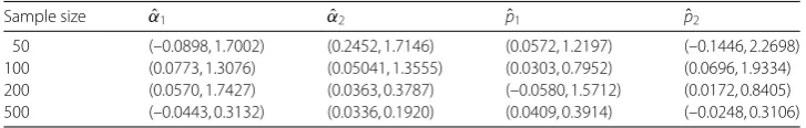
50 (–0.0898, 1.7002) (0.2452, 1.7146) (0.0572, 1.2197) (–0.1446, 2.2698)
100 (0.0773, 1.3076) (0.05041, 1.3555) (0.0303, 0.7952) (0.0696, 1.9334)
200 (0.0570, 1.7427) (0.0363, 0.3787) (–0.0580, 1.5712) (0.0172, 0.8405)
500 (–0.0443, 0.3132) (0.0336, 0.1920) (0.0409, 0.3914) (–0.0248, 0.3106)
3 Simulation studies
In this section we present some simulation study.
3.1 Empirical results for unknown parameters
We consider the following two models:
Model I: α1= 0.6,α2= 0.8,p1= 0.4,p2= 0.5withλ= 1andλ= 2.
Model II: α1= 0.7,α2= 0.5,p1= 0.3,p2= 0.6withλ= 1andλ= 2.
For both models, we obtain the empirical bias (Bias) and the standard error (SE) based on 500 replications for each parameter combination. These simulation studies are given in Table 1, 2, 3 and4, respectively, where the format (Bias, SE) is used; for example, (–0.02130.0389) means that the bias is –0.0213, and SE is 0.0389.
From the simulation results, we can see that the bias and standard errors are getting smaller when the sample size increasing. For smaller sample size, the standard errors are a little bigger, this may be because the true values of parameters are small and may disappear in their own stand error.
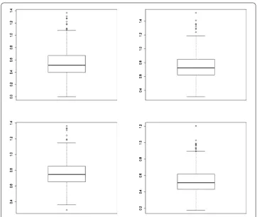
[image:6.595.118.480.297.356.2] [image:6.595.116.480.397.455.2]Figure 1The two figures in first line are the Boxplot of estimated parameterα1,α2, respectively, for Model I
withλ= 1. The two figures in second line are the Boxplot of estimated parameterp1,p2, respectively, for
Model I withλ= 1. All Boxplots are obtained with sample sizen= 500
3.2 Test for parameters
In this subsection, we consider to test the following hypotheses for Model I and II, given in Sect.3.1:
H0:α2= 0 vs. H1:α2> 0.
We report the empirical sizes for Model III and IV at a significance level 0.05 with sample sizen= 50, 100, 200, 500, respectively:
Model III: α1= 0.6,α2= 0,p1= 0.2,p2= 0.7withλ= 1andλ= 2.
Model IV: α1= 0.3,α2= 0,p1= 0.2,p2= 0.7withλ= 1andλ= 2.
The results are presented in Table5. From Table5, we can see that the empirical sizes is closed to 0.05 whennincreases.
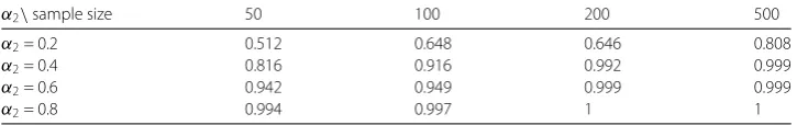
In order to investigate the power of the test, we consider the alternative hypothesis with parameter α2= 0.2, 0.6, 0.8 for Model III and IV, respectively. We report the empirical
power at a significance level 0.05 with sample sizen= 50, 100, 200, 500. The simulation results are given by Tables6–9. From these tables, we can see that the power increases monotonically when the parameterα2increases.
4 Conclusion
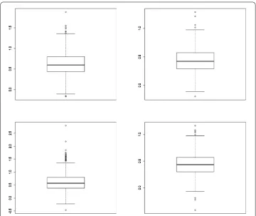
pa-Figure 2The two figures in first line are the Boxplot of estimated parameterα1,α2, respectively, for Model II
withλ= 1. The two figures in second line are the Boxplot of estimated parameterp1,p2, respectively, for
[image:8.595.117.478.80.383.2]Model II withλ= 1. All Boxplots are obtained with sample sizen= 500
Table 5 Empirical sizes
Sample size λ= 1 (III) λ= 2 (III) λ= 1 (IV) λ= 2 (IV)
50 0.076 0.076 0.084 0.09
100 0.066 0.08 0.08 0.056
200 0.058 0.046 0.056 0.074
500 0.052 0.056 0.044 0.056
Table 6 Empirical powers for Model III withλ= 1
α2\sample size 50 100 200 500
α2= 0.2 0.59 0.608 0.706 0.842
α2= 0.4 0.818 0.93 0.984 0.997
α2= 0.6 0.808 0.942 0.996 0.999
α2= 0.8 0.998 0.998 0.999 1
[image:8.595.114.481.461.517.2] [image:8.595.117.480.555.612.2]Table 7 Empirical powers for Model III withλ= 2
α2\sample size 50 100 200 500
α2= 0.2 0.684 0.686 0.682 0.846
α2= 0.4 0.864 0.936 0.976 0.999
α2= 0.6 0.905 0.954 0.998 1
[image:9.595.115.480.196.253.2]α2= 0.8 0.978 0.997 0.999 1
Table 8 Empirical powers for Model IV withλ= 1
α2\sample size 50 100 200 500
α2= 0.2 0.636 0.604 0.696 0.824
α2= 0.4 0.856 0.884 0.994 0.998
α2= 0.6 0.964 0.996 0.999 0.998
α2= 0.8 0.994 0.997 1 1
Table 9 Empirical powers for Model IV withλ= 2
α2\sample size 50 100 200 500
α2= 0.2 0.512 0.648 0.646 0.808
α2= 0.4 0.816 0.916 0.992 0.999
α2= 0.6 0.942 0.949 0.999 0.999
α2= 0.8 0.994 0.997 1 1
5 The proofs of main results
Proof of Theorem2.1 Define a random sequence{Xt(n)}n∈Zas follows:
Xt(n)= ⎧ ⎪ ⎪ ⎨ ⎪ ⎪ ⎩
0, n< 0;
t, n= 0;
θ1◦Xtn–1–1+θ2◦Xtn–2–1+t, n> 0.
(5.1)
The random vector (θ1,θ2) has a joint distribution given by (1.3) and is independent of
{t}, the random sequences used in the operatorθ1◦andθ1◦are the same for fixedt. We
first prove that the first two moments of{X(tn)}are finite. It is easy to verify that
EXt(0)=λ, EXt(1)= (β1+β2)λ+λ,
whereβ1=α1p1,β2=α2p2. Using the method of induction, we conclude that
EXt(n)=
n
i=0
(β1+β2)iλ<∞.
We have
EXt(0)
2
=E2t,EXt(1)
2
= (α1β1+α2β2)Et2+Et2+λ
β1(1 –α1) +β2(1 –α2)
[image:9.595.117.480.294.351.2]
For convenience, letA=β1(1 –α1) +β2(1 –α2) + 2λ(β1+β2)]. Then using the method of
induction, we conclude that
EXt(n)
2
=Et2 n
i=0
(α1β1+α2β2)i+Aλ
n–1
k=1
(α1β1+α2β2)n–k k–1
i=0
(β1+β2)i
<∞.
The last inequality is obtained by the fact that
α1β1+α2β2=α12p1+α22p2<p1+p1< 1, β1+β2=α1p1+α2p2<p1+p1< 1.
Next we consider the convergence of the sequence{Xt(n)}. By the definition of the sequence
{Xn
t}, we have
EXt(n)–X (n–1)
t
=Eθ1◦Xt(n–1–1)+θ2◦Xt(–2n–1)–θ1◦Xt(–1n–2)–θ2◦Xt(n–2–2)
≤Eθ1◦Xt(–1n–1)–θ1◦Xt(n–1–2)+Eθ2◦Xt(n–2–1)–θ2◦Xt(–2n–2)
=β1EXt(n–1–1)–X (n–2)
t–1 +β2EXt(n–2–1)–X (n–2) t–2 ,
where the last equality is because the operator θt1◦is the same for fixedt. Repeat the
deduction and notice thatE|X(1)t–1–Xt(0)–1|=Et, we conclude that
EXt(n)–Xt(n–1)≤(β1+β2)nEt.
Then, by the triangle inequality, we obtain, for any integersn>m,
EXt(n)–Xt(m)≤Et(n–m) n
j=m+1
(β1+β2)j,
which tends to zero asn,m→ ∞. Note that
EXt(n)–Xt(n–1) 2
=Eθ1◦Xt(n–1–1)+θ2◦Xt(–2n–1)–θ1◦Xt(–1n–2)–θ2◦Xt(n–2–2) 2
=Eθ1◦Xt(–1n–1)–θ1◦Xt(n–1–2) 2
+Eθ2◦Xt(–2n–1)–θ2◦Xt(n–2–2) 2
+ 2Eθ1◦Xt(–1n–1)–θ1◦Xt(–1n–2)θ2◦Xt(–2n–1)–θ2◦Xt(n–2–2)
≤β1(1 –α1) + 2β1
EXt(–1n–1)–Xt(–1n–2)+α1β1EX(t–1n–1)–Xt–1t(n–2) 2
+β2(1 –α2) + 2β2
EXt(n–2–1)–X(t–2n–2)+α2β2EXt(–2n–1)–Xt–2t(n–2) 2
≤ · · ·
≤(α1β1+α2β2)nEt2+BEt n–1
k=1
(α1β1+α2β2)k–1(β1+β2)n–k,
whereB=β1(1 –α1) + 2β1+β2(1 –α2) + 2β2. Then we get, for any integersn>m,
EXt(n)–Xt(m) 2≤
Et2+BEt
(n–m)
n
j=m+1
(α1β1+α2β2)j+j(β1+β2)j
,
which tends to zero asn,m→ ∞. This implies that{Xt(n)}is a Cauchy sequence. Let{Xt}
be the limit process of{X(tn)}, then the first two moments ofXtexist. Now we verify that
{Xt}satisfies (1.2). SinceXt(n) L2
−→Xt, we have, for anyt,
Eθ1◦Xt(n)–θ1◦Xt 2
=β1(1 –α1)EXt(n)–Xt+α1β1EXt(n)–Xt 2
→0.
Similarly, we can prove that for anyt
Eθ2◦Xt(n)–θ2◦Xt 2
→0.
By the uniqueness of the convergence inL2, we conclude that{Xt}satisfies (1.2).
Notice thatXt(1)=t, we know that{Xt(1)}is a strict stationary process, then, by the
in-duction method and the definition (5.1), we can see that, for eachn, the process{Xt(n)}is
strict stationary. The ergodicity can be obtained similarly as in Zhang et al. [16], we omit
the details here.
Proof of Theorem2.2 By the strict stationarity and ergodicity of the process{Xt}, adopting
the standard martingale central limit theorem, we obtain
√
n(ηˆ–η) =
1
nM
–1 1
√
nEn(η)
d
−→N0,V–1ΣV–1,
whereV=limn→∞(1/n)M,En(η) = (En1(η),En2(η),En3(η))T,Σ= (σij) is a symmetric
ma-trix with
σ11=E(Xt–β1Xt–1–β2Xt–2–λ)2X2t–1, σ22=E(Xt–β1Xt–1–β2Xt–2–λ)2Xt2–2, σ33=E(Xt–β1Xt–1–β2Xt–2–λ)2, σ21=E(Xt–β1Xt–1–β2Xt–2–λ)2Xt–1Xt–2, σ23=E(Xt–β1Xt–1–β2Xt–2–λ)2Xt–2, σ31=E(Xt–β1Xt–1–β2Xt–2–λ)2Xt–1.
Note that
√
n– 2θˆ(η) –θ=
1
n– 2
n
t=3
ZtZtT
–1
1 √
n– 2
n
t=3
Zt
Vt–ZTt θ
.
By simple calculation, we see thatZt(Vt–ZtTθ) is a martingale. Then, by the condition
E|Xt|8<∞, stationarity and ergodicity of the process{Xt}, using the martingale central
limit theorem as above, we have
√
whereΓ =E(ZtZTt),W=E((Vt–ZtTθ)2ZtZtT). Observe that
√
n– 2θ¯(ηˆ) –θ=√n– 2θ¯(ηˆ) –θˆ(η)+√n– 2θˆ(η) –θ
and
√
nθ¯(ηˆ) –θˆ(η)= 1 n n t=1
ZtZTt
–1 1 √ n n t=1 Zt
Vt(ηˆ) –Vt(η)
,
whereVt(ηˆ) is theVt(η) replaced byηwithηˆ. By a Taylor expansion, we have
Vt(ηˆ) –Vt(η) = –2
Xt–E[Xt|Ft–1]
Xt–1(βˆ1–β1) +Xt–2(βˆ2–β2) + (ˆλ–λ)
+oP
ˆη–η.
Note that 1 √ n n t=1
ZtXt–1
Xt–E[Xt|Ft–1]
(βˆ1–β1)
=√n(βˆ1–β1)
1
n
n
t=1
ZtXt–1
Xt–E[Xt|Ft–1]
.
Notice thatE[ZtXt–1(Xt–E[Xt|Ft–1])] = 0, then, by the ergodicity of the process{Xt}, we
conclude that 1 n n t=1
ZtXt–1
Xt–E[Xt|Ft–1]
→0, a.s.
Combining with the fact that√n(βˆ1–β1) converges in distribution, we have
1 √ n n t=1
ZtXt–1
Xt–E[Xt|Ft–1]
(βˆ1–β1) =oP(1).
Similarly, we can prove that
1 √ n n t=1
ZtXt–2
Xt–E[Xt|Ft–1]
(βˆ2–β2) =oP(1),
1 √ n n t=1 Zt
Xt–E[Xt|Ft–1]
(ˆ
λ–λ) =oP(1).
Therefore, we get
1 √ n n t=1 Zt
Vt(ηˆ) –Vt(η)
Again, by the ergodicity of the process{Xt}, we have
1
n
n
t=1
ZtZTt →Γ, a.s.
Thus, we can obtain the conclusion that
√
nθ¯(ηˆ) –θˆ(η)=oP(1).
Then, by the Slutsky theorem, we have
√
nθ¯(ηˆ) –θ=√nθ¯(ηˆ) –θ¯(η)+√nθˆ(η) –θ−→N0,Γ–1WΓ–1.
Therefore, we conclude that the vector (√n(θ¯(ηˆ) –θ),√n(ηˆ–η)) converges to a normal distribution with mean zero and covariance matrix
Ω= (ωij)9×9=
Γ–1WΓ–1 Γ–1ΠV–1 V–1Π Γ–1 V–1ΣV–1
,
whereΠ=E((Vt–ZtTθ)(Xt–ηTDt)ZtDTt),Dt= (Xt,Xt–1, 1)T.
Proof of Theorem2.3 We can see that the estimatorsαˆ1,αˆ2,pˆ1,pˆ1are consistent and have
asymptotic normal distribution. Specially,√n(αˆ1–α1),
√
n(αˆ2–α2) converge to normal distribution with mean zero and
variance
β2
1ω11+ (β12–θ1)2ω77+β1(β12–θ1)ω17 β4
1
,
β22ω22+ (β22–θ2)2ω88+β2(β22–θ2)ω28
β24 .
(5.2)
And√n(pˆ1–p1),
√
n(pˆ2–p2) converge to normal distribution with mean zero and variance β12(2θ12+β1)2ω77+ 4β14θ1ω11– 4β13θ1(2θ12+β1)ω17
(θ2 1 +β1)4
,
β22(2θ22+β2)2ω88+ 4β24θ2ω22– 4β23θ2(2θ22+β2)ω28
(θ22+β2)4
.
(5.3)
Proof of Corollary2.4 Observe that
ˆ
W–W= 1
n– 2
n
t=3
Vt(ηˆ) –ZtTθ¯2(ηˆ)
2
–Vt–ZtTθ2
2
ZtZTt
= 1
n– 2
n
t=3
Vt(ηˆ)2–Vt2
ZtZtT+
1
n– 2
n
t=3
ZTtθ¯2(ηˆ)
2
–ZTtθ2
2
ZtZtT
+ 1
n– 2
n
t=3
2VtZtTθ2– 2Vt(ηˆ)ZtTθ¯2(ηˆ)
:=T1+T2+T3.
Note that
T1=
1
n– 2
n
t=3
ˆ
ηT–ηTFtZtZtT whereFt= (Xt–1,Xt–2, 1).
We have
|T1| ≤ηˆT–ηT
1
n– 2
n
t=3
FtZtZtT whereFt= (Xt–1,Xt–2, 1).
By ergodicity of the process{Xt}and the fact thatηˆT P
−→η, we have
T1=oP(1).
Similarly, we have
T2=oP(1), T3=oP(1).
Similarly, we can prove that Σˆ −→P Σ,Πˆ −→P Π. The conclusion of this corollary
fol-lows.
Acknowledgements
The author thanks the editor for the guidance and help.
Funding
This research was supported by the Science and Technology Development Program of Jilin Province (Grant No. 20170101152JC).
Competing interests
The author declares to have no competing interests.
Authors’ contributions
The author read and approved the final manuscript.
Publisher’s Note
Springer Nature remains neutral with regard to jurisdictional claims in published maps and institutional affiliations.
Received: 23 September 2018 Accepted: 15 April 2019
References
1. McKenzie, E.: Some simple models for discrete variate time series. Water Resour. Bull.21, 645–650 (1985) 2. Al-Osh, M.A., Alzaid, A.A.: First order integer-valued autoregressive (INAR(1)) processes. J. Time Ser. Anal.8, 261–275
(1987)
3. Alzaid, A.A., Al-Osh, M.A.: First order integer-valued autoregressive (INAR(1)) processes: distributional and regression properties. Stat. Neerl.42, 53–61 (1988)
4. Zheng, H., Basawa, I.V., Datta, S.: First-order random coefficient integer-valued autoregressive processes. J. Stat. Plan. Inference173, 212–229 (2007)
5. Zheng, H., Basawa, I.V., Datta, S.: Inference for pth-order random coefficient integer-valued autoregressive processes. J. Time Ser. Anal.27, 411–440 (2006)
6. Zhang, H., Wang, D., Zhu, F.: Empirical likelihood for first-order random coefficient integer-valued autoregressive processes. Commun. Stat., Theory Methods40, 492–509 (2011)
7. Zhang, H., Wang, D., Zhu, F.: Empirical likelihood inference for random coefficient INAR(p) process. J. Time Ser. Anal.
32, 195–223 (2011)
9. Nedényi, F., Pap, G.: Iterated scaling limits for aggregation of random coefficient AR(1) and INAR(1) processes. Stat. Probab. Lett.118, 16–23 (2016)
10. Ding, X., Wang, D.: Empirical likelihood inference for INAR(1) model with explanatory variables. J. Korean Stat. Soc.
45(4), 623–632 (2016)
11. Nasti´c, A.S., Risti´c, M.M.: Some geometric mixed integer-valued autoregressive (INAR) models. Stat. Probab. Lett.22, 805–811 (2012)
12. Lawrance, A.J., Lewis, P.A.W.: Modelling and residual analysis of nonlinear autoregressive time series in exponential variables. J. R. Stat. Soc. B47, 165–202 (1985)
13. Dewald, L.S., Lewis, P.A.W.: A new Laplace second-order autoregressive. IEEE Trans. Inf. Theory31, 645–651 (1985) 14. Karlsen, H., Tjøstheim, D.: Consistent estimates for the NEAR(2) and NLAR(2) time series models. J. R. Stat. Soc. B50(2),
313–320 (1988)
15. Zhao, Z., Hu, Y.: Statistical inference for first-order random coefficient integer-valued autoregressive processes. J. Inequal. Appl.2015, 359 (2015)https://doi.org/10.1186/s13660-015-0886-y