A semi smoothing augmented Lagrange multiplier algorithm for low rank Toeplitz matrix completion

R E S E A R C H

Open Access

A semi-smoothing augmented Lagrange

multiplier algorithm for low-rank Toeplitz

matrix completion

Ruiping Wen

_{, Shuzhen Li}

_{and Yonghong Duan}

*_{Correspondence:[email protected]}

1_{Key Laboratory of Engineering &} Computing Science, Shanxi Provincial Department of Education/Department of Mathematics, Taiyuan Normal University, Jinzhong, P.R. China Full list of author information is available at the end of the article

Abstract

The smoothing augmented Lagrange multiplier (SALM) algorithm is a generalization of the augmented Lagrange multiplier algorithm for completing a Toeplitz matrix, which saves computational cost of the singular value decomposition (SVD) and approximates well the solution. However, the communication of numerous data is computationally demanding at each iteration step. In this paper, we propose an accelerated scheme to the SALM algorithm for the Toeplitz matrix completion (TMC), which will reduce the extra load coming from data communication under reasonable smoothing. It has resulted in a semi-smoothing augmented Lagrange multiplier (SSALM) algorithm. Meanwhile, we demonstrate the convergence theory of the new algorithm. Finally, numerical experiments show that the new algorithm is more effective/economic than the original algorithm.

Keywords: Toeplitz matrix; Completion; Augmented Lagrange multiplier; Data communication

1 Introduction

Completing a low-rank matrix from a subset of its entries has been a hot problem re-cently, first introduced by [8], that has arisen in a wide variety of practical contexts across all disciplines of engineering and computational science such as model reduction [19], ma-chine learning [1,2], control [22], pattern recognition [12], imaging inpainting [3], video denoising [16], computer vision [28], and so on. Despite matrix completion (MC) requir-ing the global solution of a non-convex objective, there are many computational efficient algorithms which are effective for a broad class of matrices. The problem has received in-tensive research from both theoretical and algorithmic aspects, see, e.g., [4–11,13–18,21, 23,26,27,29–32,34,35], and the references therein for partial review. It is well known that the mathematical model of the MC problem is of the following form:

min

A∈Rm×nA∗,

subject toPΩ(A) =PΩ(M),

(1.1)

where the matrixM∈Rm×n_{is an underlying matrix to be completed,Ωis a random subset} of indices for the available entries, andPΩ is the associated sampling orthogonal projec-tion operator which acquires only the entries indexed byΩ⊂ {1, 2, . . . ,m} × {1, 2, . . . ,n}.

In the current MC problems, the matrixMis of special structure in general. Therefore, much attention has been paid to the completion of Toeplitz and Hankel matrices in recent years [20,24,25,30,32]. Many scholars have conducted in-depth research on the special structure, property, and application of the Toeplitz and Hankel matrices; for example, nu-clear norm minimization for the low-rank Hankel matrix reconstruction problem under the random Gaussian sampling model is investigated in [7]. In addition, Hankel matrix re-constitution in the sense of minimizing the nuclear norm with non-uniform sampling of entries is researched in [11]. To make full use of the special structure of a Toeplitz matrix, a mean value algorithm is presented in [30]; the modified Lagrange multiplier (MALM) algorithm [31] and the smoothing augmented Lagrange multiplier (SALM) algorithm [34] are also proposed. Therefore, the Toeplitz matrix completion (TMC) is one of the most important MC problems and has attracted a large amount of attention recently. As is well known, ann×nToeplitz matrix is of the following form:

T= (tj–i)ni,j=1=

⎛ ⎜ ⎜ ⎜ ⎜ ⎜ ⎜ ⎜ ⎝

t0 t1 · · · tn–2 tn–1

t–1 t0 · · · tn–3 tn–2

..

. ... . .. ... ... t–n+2 t–n+3 · · · t0 t1

t–n+1 t–n+2 · · · t–1 t0

⎞ ⎟ ⎟ ⎟ ⎟ ⎟ ⎟ ⎟ ⎠

∈Tn×n_⊂Rn×n_{, (1.2)}

which is determined by 2n– 1 entries, say, the first row and the first column. Explicitly seeking the lowest rank Toeplitz matrix consistent with the known entries is mathemati-cally considered as

min

A∈Tn×nA∗,

subject toH◦A=M,

(1.3)

where “◦” is the Hadamard product,H= (Hij)∈Rn×nis the weighted matrix with entries Hij= 1 forj–i∈Ω⊂ {–n+ 1, . . . ,n– 1}andHij= 0 for any other (i,j),M= (Mij)∈Tn×nis the underlying Toeplitz matrix to be completed, namelyMij= 0 forj–i∈/Ω.

The SALM algorithm switches the iteration matrix into the Toeplitz structure at each iteration step by the smoothing operator, which saves computational cost of the singular value decomposition and approximates well the solution. Unfortunately, numerous data have to be shifted at each iteration step in the process of implementing this algorithm. However, there is a cost, sometimes relatively great, associated with the moving of data. The control of memory traffic is crucial to performance in many computers.

These factors motivated us to reduce the traffic jam of data, resulting in a semi-smoothing augmented Lagrange multiplier (SSALM) algorithm based on the selecting technique of the optimal parameterω(k)_{at each of the five iteration steps in [33].}

communication for the ALM algorithm. We can see that the CPU of SSALM algorithm is reduced to 30.44% from the numerical experiments.

The rest of this paper is organized as follows. Some preliminaries are provided in Sect.2. Section3presents the semi-smoothing augmented Lagrange multiplier (SSALM) algo-rithm after giving an outline of the ALM algoalgo-rithm, the dual approach, and the SALM algorithm. The convergence property of the SSALM algorithm is constructed in Sect.4. We report the numerical results to indicate the effectiveness of the SSALM algorithm in Sect.5. Finally, we end the paper with the concluding remarks in Sect.6.

2 Preliminaries

This section is devoted to some of the necessary notations and preliminaries.Rm×n de-notes the set ofm×nreal matrices,Tn×n_{is the set ofn×nreal Toeplitz matrices. The} nuclear norm of a matrix Ais denoted byA∗, and the Frobenius norm AF is the maximum absolute value of the matrix entries of a matrixA.AT is used to express the transpose of a matrixA∈Rn×n,rank(A) is equal to the rank of a matrixA, andtr(A) rep-resents the trace ofA. The standard inner product between two matrices is denoted by X,Y=tr(XT_{Y). ForA= (a}

ij)∈Rm×n,B= (bij)∈Rm×n, their Hadamard productA◦Bis anm×nmatrix whose (i,j) entry is theaijbij, i.e.,A◦B= (aijbij)∈Rm×n.

The singular value decomposition (SVD) of a matrixA∈Rm×nofr-rank is defined by A=UΣrVT, Σr=diag(σ1,σ2, . . . ,σr),

whereU∈Rm×r _{andV ∈R}n×r _{are column orthonormal matrices, andσ}

1≥σ2≥ · · · ≥

σr> 0.

Definition 2.1 (Singular value thresholding operator [6]) For eachτ ≥0, the singular

value thresholding operatorDτ is defined as follows:

Dτ(A) :=UDτ(Σ)VT, Dτ(Σ) =diag

{σi–τ}+ ,

where

A=UΣrVT∈Rm×n, {σi–τ}+=

⎧ ⎨ ⎩

σi–τ, ifσi>τ,

0, ifσi≤τ.

In= (e1,e2, . . . ,en)∈Rn×ndenotes then×nidentity matrix andZn= (e2,e3, . . . ,en, 0)∈ Rn×n_{is called the shift matrix. It is clear that}

Zr_n=

⎧ ⎨ ⎩

(_IO O

n–rO), 1 <r<n, O, r≥n,

where “O” stands for a zero-matrix. Thus, a Toeplitz matrixT∈Tn×n_{, shown in (1.2), can} be written as a linear combination of these shift matrices, that is,

T= n–1

l=1

t–lZln+ n–1

l=0

tl

Ω⊂ {–n+ 1, . . . ,n– 1}is an indices set of observed diagonals of a Toeplitz matrixM∈ Tn×n_{, Ω}¯ _{is the complementary set ofΩ. For any Toeplitz matrixA∈T}n×n_{, the vector} vec(A,α) denotes theαth diagonal ofA,α= –n+ 1, –n+ 2, . . . ,n– 1, that is to say,

vec(H◦A,α) =

⎧ ⎨ ⎩

vec(A,α), α∈Ω,

0, α∈/Ω, (0 is a zero-vector).

Definition 2.2(Toeplitz structure smoothing operator [34]) For any matrixA= (aij)∈ Rn×n_{, the Toeplitz structure smoothing operatorT is defined as follows:}

T(A) := n–1

l=1

˜ a–lZln+

n–1

l=0

˜ al

ZT_n l, (2.1)

wherea˜α=αA min₊

αAmax

2 ,α= –n+ 1, –n+ 2, . . . ,n– 1 with

αAmin= min

i,j∈{1,2,...,n}{aij,i–j=α}, and αA

max

= max

i,j∈{1,2,...,n}{aij,i–j=α}.

It is clear thatT(A) is a Toeplitz matrix derived from the matrixA. Namely, anyA∈Rn×n can be changed into a Toeplitz structure via the smoothing operatorT(·).

3 Algorithms

First of all in this section, for completeness as well as for the purpose of comparison, we briefly review and summarize some relative algorithms for approximately minimizing the nuclear norm of a matrix under convex constraints.

Since the matrix completion problem is closely connected to the robust principal com-ponent analysis (RPCA) problem, then it can be formulated in the same way as RPCA, an equivalent problem of (1.1) can be considered as follows.

As E will compensate for the unknown entries ofM, the unknown entries ofMare simply set as zeros. Suppose that the given data are arranged as the columns of a large matrixM∈Rm×n_{. The mathematical model for estimating the low-dimensional subspace} is to find a low-rank matrix A∈Rm×n _{such that the discrepancy betweenAandMis} minimized, leading to the following constrained optimization:

min

A,E∈Rm×nA∗,

subject toA+E=M,PΩ(E) = 0,

(3.1)

whereEwill compensate for the unknown entries ofM, the unknown entries ofM∈Rm×n are simply set as zeros. AndPΩ:Rm×n→Rm×nis a linear operator that keeps the entries inΩunchanged and sets those outsideΩ(say, inΩ) zeros.

3.1 The dual algorithm

The dual algorithm proposed in [10] tackles problem (3.1) via its dual. That is, one first solves the dual problem

max

Y M,Y, subject toJ(Y)≤1,

for the optimal Lagrange multiplierY, where

J(Y) =maxY2,λ–1Y∞ . (3.3)

A steepest ascend algorithm constrained on the surface{Y|J(Y) = 1}can be adopted to solve (3.2), where the constrained steepest ascend direction is obtained by projectingM onto the tangent cone of the convex body{Y|J(Y)≤1}. It turns out that the optimal so-lution to the primal problem (3.1) can be obtained during the process of finding the con-strained steepest ascend direction.

3.2 The augmented Lagrange multiplier algorithm

The augmented Lagrange multiplier (ALM) algorithm was proposed in [18] for solving a convex optimization (1.1). It should be described subsequently.

It is famous that the partial augmented Lagrangian function of problem (3.1) is

L(A,E,Y,μ) =A∗+Y,M–A–E+μ

2M–A–E

2

F. (3.4)

Hence, the augmented Lagrange multiplier algorithm is designed as follows.

Algorithm 3.1([18]) Given a sampled setΩ, a sampled matrixD=PΩ(M),μ0> 0,ρ> 1.

Given also two initial matricesY0= 0,E0= 0.k:= 0.

1. Compute the SVD of the matrix(D–Ek+μ–1k Yk):

[Uk,Σk,Vk] =svd

D–Ek+μ–1k Yk ;

2. Set

Ak+1=UkDμ–1_k (Σk)VkT,

solveEk+1=arg minPΩ(E)=0L(Ak+1,E,Yk,μk),

Ek+1=PΩ¯

D–Ak+1+μ–1k Yk ;

3. IfD–Ak+1–Ek+1F/DF<1andμkEk+1–EkF/DF<2, stop; otherwise, go

to the next step;

4. SetYk+1=Yk+μk(D–Ak+1–Ek+1).

IfμkEk+1–EkF/DF<2, setμk+1=ρμk; otherwise, go to Step 1.

3.3 The smoothing augmented Lagrange multiplier algorithm

In this subsection, we make mention of a stepped-up scheme for the TMC problem. The smoothing augmented Lagrange multiplier (SALM) approach employs the smoothing op-eratorT (see (2.1)) to approximate a matrix generated in thekth iteration so that the cur-rent approximation is of a Toeplitz structure.

Then our problem can be expressed as the following convex programming:

min

A,E∈Tn×nA∗,

subject to A+E=PΩ(M), PΩ(E) = 0,

(3.5)

whereM∈Tn×n_{is a real Toeplitz matrix, andΩ⊂ {–n+ 1, . . . ,n– 1}.} LetD=PΩ(M). Then the partial augmented Lagrangian function is

L(A,E,Y,μ) =A∗+Y,D–A–E+μ

2D–A–E

2

F, (3.6)

whereY∈Rn×n_.

Algorithm 3.2([34]) Given a sampled setΩ, a sampled matrixD,μ0> 0,ρ> 1. Given

also two initial matricesY0= 0,E0= 0.k:= 0.

1. Compute the SVD of the matrix(D–Ek+μ–1k Yk)using the Lanczos method

[Uk,Σk,Vk] =lansvd

D–Ek+μ–1k Yk ;

2. Set

Xk+1=UkDμ–1_k (Σk)VkT,

compute for smoothinga˜α=

αXmink+1+αXkmax+1

2 ,α∈ {–n+ 1, –n+ 2, . . . ,n– 1}, and

Ak+1=T(Xk+1) =

n–1

l=1

˜ a–lZln+

n–1

l=0

˜ al

Z_nT l,

Ek+1=PΩ¯

D–Ak+1+μ–1k Yk ;

3. IfD–Ak+1–Ek+1F/DF<1andμkEk+1–EkF/DF<2, stop; otherwise, go

to the next step;

4. SetYk+1=Yk+μk(D–Ak+1–Ek+1).

IfμkEk+1–EkF/DF<2, setμk+1=ρμk; otherwise, go to Step 1.

It is reported that the convergence speed of the SALM algorithm is greater than that of the ALM and APG algorithms. A merit of smoothing is that the fast SVD procedure can be utilized to reduce the computation.

3.4 The semi-smoothing augmented Lagrange multiplier algorithm

In this subsection, we propose a semi-smoothing augmented Lagrange multiplier algo-rithm based on the ALM and SALM algoalgo-rithms for the TMC problem. The new algoalgo-rithm consists of two stages: one is– 1 iterations by the ALM scheme, which is free moving of data; another is theth smoothing by the SALM procedure, which is keeping the iteration matrix as a Toeplitz structure.

Now, the semi-smoothing augmented Lagrange multiplier (SSALM) algorithm will be presented in the following.

Algorithm 3.3(SSALM algorithm)

Input:A sampled setΩ, a sampled matrixD,Y0,0= 0,E0,0= 0; parametersμ0> 0,ρ> 1,

> 1,1,2.

Letk:= 0,q:= 1,q= 1, 2, . . . ,– 1.

Repeat:

1. – 1iterations.

(1) Compute the SVD of the matrix(D–Ek,q+μ–1_k,qYk,q):

[Uk,q,Σk,q,Vk,q] =lansvd

D–Ek,q+μ–1k,qYk,q ;

(2) Set

Xk+1,q+1=Uk,qDμ_k–1_,q(Σk,q)VkT,q,

Ek+1,q+1=PΩ¯

D–Xk+1,q+1+μ–1k,qYk,q ;

(3) IfD–Xk+1,q+1–Ek+1,q+1F/DF<1andμk,qEk+1,q+1–Ek,qF/DF <2,

stop; otherwise, go to the next step;

(4) SetYk+1,q+1=Yk,q+μk,q(D–Xk+1,q+1–Ek+1,q+1),μk+1,q+1=ρμk,q; otherwise, go

to step (1); 2. th smoothing.

(1) Compute the SVD of the matrix(D–Ek,+μ–1_k,Yk,):

[Uk,,Σk,,Vk,] =svd

D–Ek,+μ–1k,Yk, ;

(2) Set

Xk+1,=Uk,Dμ–1_k,(Σk,)V_kT_,,

compute the factors of smoothinga˜α=

αXmink+1,+αXkmax+1,

2 ,α= –n+ 1, –n+ 2, . . . ,

n– 1, and set

Ak+1,=T(Xk+1,) = n–1

l=1

˜ a–lZnl+

n–1

l=0

˜ al

Z_nT l.

Update

Ek+1,=PΩ¯

3. IfD–Ak+1,–Ek+1,F/DF<1andμk,Ek+1,–Ek,F/DF<2, stop;

otherwise, go to the next step;

4. SetYk+1,q+1=Yk,q+μk,q(D–Ak+1,q+1–Ek+1,q+1).

Ifμk,qEk+1,q+1–Ek,qF/DF<2, setμk+1,q+1=ρμk,q; otherwise, go to Step 1.

In fact, Algorithm3.3includes the above Algorithm3.2as a special case if= 1. Obvi-ously, the algorithm is an acceleration of the SALM algorithm in [34].

4 Convergence analysis

This section will analyze the convergence of Algorithm3.3.

Let (A,¨ E) be the solution of model (3.5) and¨ Y¨ be that of the optimal problem (3.2). We provide some lemmas in the following firstly.

Lemma 4.1([8]) Let A∈Rm×n_{be an arbitrary matrix and UΣV}T_{be its SVD.Then the} set of subgradients of the nuclear norm of A is given by

∂A∗=UVT+W:W∈Rm×n,UTW= 0,WV= 0,W2≤1

.

Lemma 4.2([18]) Ifμkis nondecreasing,then each entry of the following series is nonneg-ative and their sum is finite,i.e.,

+∞

k=1

μk–1

Yk+1–Yk,Ek+1–Ek+Ak+1–A,¨ Yˆk+1–Y¨ +Ek+1–E,¨ Yk+1–Y¨

< +∞. (4.1)

Lemma 4.3([18]) The sequences{ ¨Yk},{Yk},and{ ˆYk}are all bounded,whereYˆk=Yk+1+

μk–1(D–Ak–Ek–1).

Lemma 4.4 The sequence{Yk,q}generated by Algorithm3.3is bounded.

Proof LetB=μk,q(D–Ek,q+μk–1,qYk,q–Xk+1,q+1),T(B) =

n–1

l=1 b˜–lZnl+

n–1

l=0 b˜l(ZTn)l, defined as (2.1).

First of all, we indicate thatYk,q,Ek,q,k= 1, 2, . . . ,q= 1, 2, . . . ,– 1, are all the Toeplitz matrices. Clearly,Y0,0= 0,E0,0= 0 are both smoothed into a Toeplitz structure. Suppose

thatYk,q,Ek,q are both the Toeplitz matrices, so isEk+1,q+1=PΩ¯(D–Xk+1,q+1+μ–1k,qYk,q). Thus,Yk+1,q+1is a Toeplitz matrix also because of Step 4 in Algorithm3.3.

Yk+1,q+1=Yk,q+μk,q(D–Ak+1,q+1–Ek+1,q+1)

=Yk,q+μk,q(D–Ak+1,q+1–Ek,q) +μk,q(Ek,q–Ek+1,q+1).

Moreover,

μk,q(Ek,q–Ek+1,q+1) =μk,qPΩ¯

Ek,q–

D–Ak+1,q+1+μ–1k,qYk,q

=μk,qPΩ¯

Ek,q–

D–T(Xk+1,q+1) +μ–1k,qYk,q

=μk,qPΩ¯

Ek,q–

D–TD–Ek,q+μ–1k,qYk,q–μ–1k,qB +μ–1k,qYk,q

=μk,qPΩ¯

Ek,q–

D–D–Ek,q+μ–1k,qYk,q–μ–1k,qT(B) +μ–1k,qYk,q

=PΩ¯T(B).

It is clear that by Steps 1–2 in Algorithm3.3we have

D–Ek,q+μ–1k,qYk,q=Uˇk,qΣˇk,qVˇkT,q+U˜k,qΣ˜k,qV˜kT,q,

whereUˇk,q,Vˇk,qare the singular vectors associated with singular values that are more than

1

μk,q andU˜k,q,V˜k,qare those associated with singular values that are less than or equal to 1

μk,q, the elements of the diagonal matrixΣˇk,qare more than 1

μk,q, and those of the diagonal

matrixΣ˜k,q are less than or equal to μ1_k,q. Hence, it is drawn thatAk+1,q+1=Uˇk,q(Σˇk,q–

μ–1_k,qI)Vˇ_kT_,q, and

BF =μk,q

D–Ek,q+μ–1k,qYk,q–Ak+1,q+1 _F

=μk,q

μ–1_k,qUˇk,qVˇkT,q+U˜k,qΣ˜k,qV˜kT,q F

=Uˇk,qVˇkT,q+μk,qU˜k,qΣ˜k,qV˜kT,qF ≤√n.

We can obtain hence thatYk,q+μk,q(D–Ak+1,q+1–Ek,q)∈∂Ak+1,q+1∗from Lemmas4.2

and4.3.

It is known that, forAk+1,q+1=UΣVT, by Lemma4.1,

∂Ak+1,q+1∗=

UVT+W:W∈Rn×n,UTW= 0,WV= 0,W2≤1

.

We also have

UVT+W2_F=trUVT+W TUVT+W =trVVT+WTW ≤n.

Therefore, the following inequalities can be obtained:

Yk,q+μk,q(D–Ak+1,q+1–Ek,q)_F≤ √

n

and

_PΩ¯

T(B) _F≤T(B))_F≤ BF≤ √

n.

It is evident that the sequence{Yk,q}is bounded.

Theorem 4.1 Suppose thatAk+1,q+1–Ak,q,D–Ak+1,q+1–Ek,q ≥0,then the sequence{Ak,q} converges to the solution of(3.5)whenμk,q→ ∞and+k=1∞μ–1k,q= +∞.

Proof It is true that

lim

k→∞(D–Ak+1–Ek+1) = 0

Let (A,¨ E) be the solution of (3.5). Then¨ Ak+1,q+1,Yk+1,q+1,Ek+1,q+1, k= 1, 2, . . . , are all

Toeplitz matrices sinceA¨+E¨=D. We prove first that

Ek+1,q+1–E¨ 2F+μk–2,qYk+1,q+1–Y¨ 2F

=Ek,q–E¨F2–Ek+1,q+1–Ek,q2F+μ–2k,qYk,q–Y¨2F

–μ–2_k,qYk+1,q+1–Yk,q2F– 2μ–1k,qAk+1,q+1–A,¨ Yˆk+1,q+1–Y,¨ (4.2)

whereYˆk+1,q+1=Yk,q+μk,q(D–Ak+1,q+1–Ek,q),Y¨is the optimal solution to the dual problem (3.2).

Ek,q–E¨ 2F =PΩ¯(Ek,q–E)¨

2

F

=PΩ¯(Ek+1,q+1–E¨–Ek+1,q+1+Ek,q)

2

F

=PΩ¯(Ek+1,q+1–E)¨ 2_F+PΩ¯(Ek+1,q+1–Ek,q)2_F – 2PΩ¯(Ek+1,q+1–E),¨ PΩ¯(Ek+1,q+1–Ek,q)

=Ek+1,q+1–E¨ 2F+Ek+1,q+1–Ek,q2F

+ 2μ–1_k,qPΩ¯(Ak+1,q+1–A),¨ Yˆk+1,q+1–Y¨

.

We obtain the following result with the same analysis:

μ–2_k,qYk,q–Y¨2F=μ–2k,qPΩ(Yk,q–Y¨)

2

F

=μ–2_k,qPΩ(Yk+1,q+1–Y¨) 2

F+μ

–2

k,qPΩ(Yk+1,q+1–Yk,q)

2

F

– 2μ–1_k,qPΩ(Yk+1,q+1–Y¨),PΩ(Yk+1,q+1–Yk,q)

=μ–2_k,qYk+1,q+1–Y¨ 2F+μ–2k,qYk+1,q+1–Yk,q2F

+ 2μ–1_k,qPΩ(Ak+1,q+1–A),¨ Yˆk+1,q+1–Y¨

.

Then

min

A∈Tm×nμA∗+

1

2PΩ(A–M)

2

F (4.3)

holds true.

The sum ∞_k=1μ–1_k,qAk,q –A,¨ Yˆk,q – Y¨ < +∞ and Ek,q –E¨2 +μ_k–2_,qYk,q –Y¨2 is nonincreasing since A∗ is a convex function and Yˆk+1,q+1 ∈ ∂A∗, Ak+1,q+1 – A,¨

ˆ

Yk+1,q+1–Y ≥¨ 0. On the other hand, the following are true by Algorithm3.3:

Yk,q,Ek,q–E¨ = 0 and ¨Y,Ek,q–E¨ = 0.

Therefore, by the same idea of Theorem 2 in [18], it is obtained thatA¨ is the solution of

(3.5).

Proof By the definition ofT(X), we have_i,j(xij–x˜ij) = 0,i,j= 1, 2, . . . ,n. SinceY is a Toeplitz matrix andyα=yij,α=i–j,i,j= 1, 2, . . . ,n, then

X–T(X),Y= n

i=1

n

j=1

(xij–x˜ij)yji

= n–1

l=1

y–l(xij–x˜ij) + n–1

l=0

yl(xij–x˜ij)

= 0.

Theorem 4.3 In Algorithm3.3,Ak,qis a Toeplitz matrix generated by Xk,q,then

Ak,q–A¨F<Xk,q–A¨F

is true withA being the solution of¨ (3.5).

Proof

Xk,q–A¨2F =Xk,q–Ak,q+Ak,q–A¨2F

=Xk,q–Ak,q,Xk,q–Ak,q+ 2Xk,q–Ak,q,Ak,q–A¨

+Ak,q–A,¨ Ak,q–A¨

=Xk,q–Ak,qF2+Ak,q–A¨ 2F.

Thus,Ak,q–A¨ F<Xk,q–A¨ Fholds true.

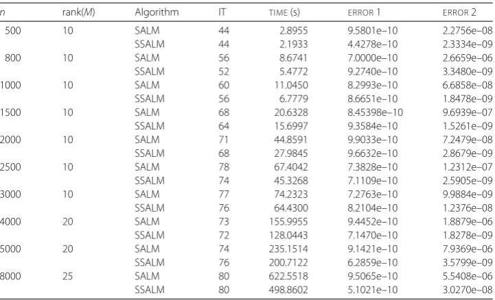
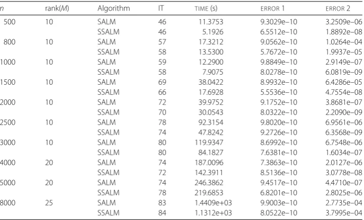
5 Numerical experiments

In this section we report some original numerical results of two algorithms (SALM, SSALM) for some n×n matrices with different ranks. All the experiments are con-ducted on the same workstation with an Intel(R) Core(TM) i7-6700 CPU @ 3.40 GHz that has 16 GB memory and 16-bit operating system, running Windows 7 and Matlab (vi-sion 2016a). We analyze and compare iteration numbers (IT), computing time in seconds (time(s)), deviation (error 1, error 2), and ratio which are defined in the following. It can be seen that the SSALM algorithm proposed in this study is highly effective compared with the SALM algorithm.

error 1 =A+E–DF DF

, error 2 = A–MF MF

,

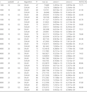
ratio =the CPU of the SSALM algorithm

the CPU of the SALM algorithm ×100%.

In the experiments,M∈Tn×n_{represents an uncompleted Toeplitz matrix, the sampling} densityp=m/(2n– 1), wheremis the number of the known diagonal entries. By the way, p∈ {0.3, 0.4, 0.5, 0.6}here. Due to the special structure of a Toeplitz matrix, we have 0≤ m≤2n– 1. The SALM and SSALM algorithms share the same values of all parameters, say,τ0= 1/D2,δ= 1.2172 + 1.8588m/n2,1= 10–9,2= 5×10–6. In the test of the SSALM

Table 1 Comparison between SALM and SSALM forp= 0.6

n rank(M) Algorithm IT TIME(s) ERROR1 ERROR2

500 10 SALM 44 2.6563 8.2372e–10 1.0363e–07

SSALM 42 1.8853 9.2608e–10 1.9658e–09

800 10 SALM 54 5.9456 8.1138e–10 8.2779e–09

SSALM 52 5.0976 5.6384e–10 7.6367e–09

1000 10 SALM 57 8.2474 8.9636e–10 4.1947e–09

SSALM 58 6.3207 7.9333e–10 1.9217e–09

1500 10 SALM 64 16.7198 9.5636e–10 2.1154e–09

SSALM 64 15.0399 9.1550e–10 1.0551e–09

2000 10 SALM 71 31.7924 9.4056e–10 7.5879e–08

SSALM 68 26.8256 8.1847e–10 2.3201e–08

2500 10 SALM 71 47.3399 7.0194e–10 1.5048e–08

SSALM 72 42.5214 9.8809e–10 2.6892e–09

3000 10 SALM 77 70.2107 6.7658e–10 2.4626e–09

SSALM 76 60.6145 6.9232e–10 1.1348e–09

4000 20 SALM 74 146.3660 6.5154e–10 5.1684e–05

SSALM 72 129.2216 5.3346e–10 1.4304e–09

5000 20 SALM 74 220.6386 9.9475e–10 2.1943e–08

SSALM 74 198.3210 5.5006e–10 1.8351e–09

8000 25 SALM 78 550.5427 9.2197e–10 3.6735e–09

SSALM 80 471.4695 5.5647e–10 1.5932e–09

Table 2 Comparison between SALM and SSALM forp= 0.5

n rank(M) Algorithm IT TIME(s) ERROR1 ERROR2

500 10 SALM 44 2.8955 9.5801e–10 2.2756e–08

SSALM 44 2.1933 4.4278e–10 2.3334e–09

800 10 SALM 56 8.6741 7.0000e–10 2.6659e–06

SSALM 52 5.4772 9.2740e–10 3.3480e–09

1000 10 SALM 60 11.0450 8.2993e–10 6.6858e–08

SSALM 56 6.7779 8.6651e–10 1.8478e–09

1500 10 SALM 68 20.6328 8.45398e–10 9.6939e–07

SSALM 64 15.6997 9.3584e–10 1.5261e–09

2000 10 SALM 71 44.8591 9.9033e–10 7.2479e–08

SSALM 68 27.9845 9.6632e–10 2.8679e–09

2500 10 SALM 78 67.4042 7.3828e–10 1.2312e–07

SSALM 74 45.3268 7.1109e–10 2.5905e–09

3000 10 SALM 77 74.2323 7.2763e–10 9.9884e–09

SSALM 76 64.4300 8.2104e–10 1.2376e–08

4000 20 SALM 73 155.9955 9.4452e–10 1.8879e–06

SSALM 72 128.0443 7.1470e–10 1.8278e–09

5000 20 SALM 74 235.1514 9.1421e–10 7.9369e–06

SSALM 76 200.7122 6.2859e–10 3.5799e–09

8000 25 SALM 80 622.5518 9.5065e–10 5.5408e–06

SSALM 80 498.8602 5.1021e–10 3.0270e–08

The experimental results of two algorithms are presented in Tables1–6. From the tables, two algorithms can successfully compute an approximate solution of the prescriptive stop condition for all the test matrixM. And computing time of our SSALM algorithm in far less than that of the SALM algorithm. In particular, compared with the cost of the SALM algorithm, we can find that the cost of the SSALM algorithm is decreased up to 30.44%. The “ratio” in Tables5–6can show this effectiveness.

6 Concluding remarks

interdepen-Table 3 Comparison between SALM and SSALM forp= 0.4

n rank(M) Algorithm IT TIME(s) ERROR1 ERROR2

500 10 SALM 45 7.8497 6.8884e–10 5.3595e–06

SSALM 44 2.3892 5.3103e–10 2.3267e–09

800 10 SALM 54 7.4948 9.3427e–10 2.1464e–06

SSALM 54 5.9618 8.9128e–10 1.5780e–08

1000 10 SALM 58 9.9528 9.7372e–10 3.2663e–05

SSALM 56 7.2641 9.7968e–10 2.4662e–09

1500 10 SALM 67 25.3226 9.8741e–10 2.7106e–06

SSALM 64 16.1484 9.0982e–10 1.5210e–09

2000 10 SALM 70 34.6083 8.4557e–10 1.8757e–07

SSALM 70 29.7298 6.4346e–10 1.7874e–09

2500 10 SALM 76 54.5748 7.1288e–10 8.4514e–08

SSALM 74 46.5716 4.9981e–10 1.6792e–09

3000 10 SALM 78 84.9121 5.3019e–10 2.2285e–06

SSALM 76 66.0761 9.2876e–10 1.1697e–09

4000 20 SALM 73 164.7655 8.6946e–10 7.3598e–06

SSALM 72 144.5329 5.1358e–10 1.4439e–09

5000 20 SALM 75 251.7641 8.9821e–10 7.9543e–08

SSALM 76 203.3167 8.3168e–10 3.4049e–08

8000 25 SALM 79 598.8095 9.5617e–10 3.7230e–08

SSALM 80 530.8533 4.9436e–10 1.2710e–09

Table 4 Comparison between SALM and SSALM forp= 0.3

n rank(M) Algorithm IT TIME(s) ERROR1 ERROR2

500 10 SALM 46 11.3753 9.3029e–10 3.2509e–06

SSALM 46 5.1926 6.5512e–10 1.8892e–08

800 10 SALM 57 17.3212 9.0562e–10 1.0264e–04

SSALM 58 13.5300 5.7672e–10 1.9937e–05

1000 10 SALM 59 12.2900 9.8849e–10 2.9149e–07

SSALM 58 7.9075 8.0278e–10 6.0819e–09

1500 10 SALM 69 38.0422 8.9932e–10 6.4286e–05

SSALM 66 17.6928 5.5536e–10 4.7554e–08

2000 10 SALM 72 39.9752 9.1752e–10 3.8681e–07

SSALM 70 30.0543 8.0322e–10 2.2090e–09

2500 10 SALM 78 92.3154 9.8020e–10 6.9561e–06

SSALM 74 47.8242 9.2726e–10 6.3568e–09

3000 10 SALM 80 119.9347 8.6992e–10 6.7548e–06

SSALM 80 84.1827 7.6381e–10 1.6034e–07

4000 20 SALM 74 187.0096 7.3863e–10 2.0127e–06

SSALM 72 142.3911 8.5136e–10 3.0778e–08

5000 20 SALM 74 246.3862 9.4517e–10 4.4710e–07

SSALM 78 219.6853 6.8201e–10 2.8025e–06

8000 25 SALM 83 1.4409e+03 9.9003e–10 2.7735e–04

SSALM 84 1.1312e+03 8.0522e–10 3.7995e–04

conges-Table 5 The values ofRATIOfor= 2

p= 0.6 n 500 800 1000 1500 2000 2500 3000 4000 5000 8000

rank(M) 10 10 10 10 10 10 10 20 20 25

RATIO(%) 70.97 85.74 76.64 89.95 84.38 89.82 86.33 88.29 89.88 85.64

p= 0.5 n 500 800 1000 1500 2000 2500 3000 4000 5000 8000

rank(M) 10 10 10 10 10 10 10 20 20 25

RATIO(%) 75.75 63.41 61.37 76.09 62.38 67.25 86.80 82.08 85.35 80.13

p= 0.4 n 500 800 1000 1500 2000 2500 3000 4000 5000 8000

rank(M) 10 10 10 10 10 10 10 20 20 25

RATIO(%) 30.44 79.55 72.99 63.77 85.90 85.34 77.82 87.72 80.76 88.65

p= 0.3 n 500 800 1000 1500 2000 2500 3000 4000 5000 8000

rank(M) 10 10 10 10 10 10 10 20 20 25

RATIO(%) 45.65 78.11 64.34 46.51 75.18 51.81 70.19 76.14 89.16 78.51

Table 6 Comparison between SALM and SSALM for= 3

n rank(M) p Algorithm IT TIME(s) ERROR1 ERROR2 RATIO (%)

500 10 0.4 SALM 47 7.5689 5.2053e–10 3.9970e–06 71.71

SSALM 47 5.4276 3.8663e–10 3.2564e–06 1000 10 0.4 SALM 60 13.9741 8.8726e–10 2.6235e–07 61.58

SSALM 59 8.6048 9.8580e–10 9.1642e–09 1500 10 0.5 SALM 68 29.6545 9.1634e–10 4.5666e–05 63.99

SSALM 68 18.9748 8.6885e–10 4.3619e–09 1500 10 0.3 SALM 69 47.1327 9.3547e–10 6.8306e–06 65.78

SSALM 68 31.0025 9.0834e–10 2.2110e–06 2000 10 0.5 SALM 73 50.5371 8.4794e–10 3.1914e–05 59.00

SSALM 71 29.8151 9.8594e–10 8.2954e–09 2000 10 0.4 SALM 72 38.5308 6.6310e–10 9.5342e–07 75.51

SSALM 69 29.0941 9.3350e–10 3.5384e–09 3000 10 0.5 SALM 79 83.3712 9.9293e–10 1.2756e–05 76.68

SSALM 78 63.9294 6.5972e–10 2.8985e–09 3000 10 0.4 SALM 77 80.7144 8.9678e–10 2.0862e–07 83.38

SSALM 78 67.2993 9.9493e–10 7.3612e–09 3000 10 0.3 SALM 79 118.3675 9.8435e–10 9.6348e–05 81.24

SSALM 80 96.1642 7.0585e–10 1.4254e–06 4000 20 0.6 SALM 73 152.4618 8.2869e–10 1.7109e–06 75.89

SSALM 72 115.7083 8.2721e–10 2.4255e–09 4000 20 0.5 SALM 72 166.5827 9.3233e–10 1.0321e–07 74.92

SSALM 72 124.8054 7.5040e–10 2.4066e–09 4000 20 0.4 SALM 75 186.7383 9.0624e–10 7.5345e–07 73.03

SSALM 74 136.3765 8.7658e–10 1.0216e–07 5000 20 0.5 SALM 75 232.0879 9.8661e–10 5.7423e–08 80.86

SSALM 75 187.6559 9.6715e–10 2.2527e–08 5000 20 0.4 SALM 76 250.9495 8.5572e–10 1.1830e–06 83.20

SSALM 77 208.7798 9.7333e–10 7.8349e–07 5000 20 0.3 SALM 76 273.7735 9.4519e–10 6.4327e–06 86.76

SSALM 80 237.5358 5.0062e–10 8.2082e–06 8000 25 0.5 SALM 80 575.2382 9.1308e–10 5.0447e–05 82.81

SSALM 81 476.3530 7.4764e–10 4.6774e–08 8000 25 0.4 SALM 80 512.3396 9.7395e–10 6.3150e–06 97.00

SSALM 81 496.9932 7.2501e–10 9.3571e–09 8000 25 0.3 SALM 83 579.2973 7.1372e–10 1.3349e–06 90.08

SSALM 80 521.8350 9.4433e–10 6.5484e–09

Acknowledgements

The authors are very much indebted to the editor and anonymous referees for their helpful comments and suggestions which greatly improved the original manuscript of this paper. The authors also are thankful for the support from the NSF of Shanxi Province (201601D011004) and the SYYJSKC-1803.

Funding It is not applicable.

Abbreviations

MC, matrix completion; TMC, Toeplitz matrix completion; SVD, singular value decomposition; SVT, singular value thresholding; APG, accelerated proximal gradient; ALM, augmented Lagrange multiplier; MALM, modified augmented Lagrange multiplier; SALM, soothing augmented Lagrange multiplier; SSALM, semi-soothing augmented Lagrange multiplier; RPCA, robust principal component analysis; IT, iteration number; CPU, computing time.

Availability of data and materials Please contact author for data requests.

Competing interests

The authors declare that they have no competing interests.

Authors’ contributions

All authors contributed equally to the writing of this paper. All authors read and approved the final manuscript.

Author details

1_{Key Laboratory of Engineering & Computing Science, Shanxi Provincial Department of Education/Department of}

Mathematics, Taiyuan Normal University, Jinzhong, P.R. China. 2_{Department of Mathematics, Taiyuan Normal University,}

Jinzhong, P.R. China.3_{Department of Mathematics, Taiyuan University, Taiyuan, P.R. China.}

Publisher’s Note

Springer Nature remains neutral with regard to jurisdictional claims in published maps and institutional affiliations.

Received: 29 January 2019 Accepted: 19 March 2019 References

1. Amit, Y., Fink, M., Srebro, N., Ullman, S.: Uncovering shared structures in multiclass classification. In: Proceeding of the 24th International Conference on Machine Learning, pp. 17–24. ACM, New York (2007)

2. Argyriou, A., Evgeniou, T., Pontil, M.: Multi-task feature learning. Adv. Neural Inf. Process. Syst.19, 41–48 (2007) 3. Bertalmio, M., Sapiro, G., Caselles, V., Ballester, C.: Multi-task feature learning, image inpainting. Comput. Graph.34,

417–424 (2000)

4. Blanchard, J., Tanner, J., Wei, K.: CGIHT: conjugate gradient iterative hard thresholding for compressed sensing and matrix completion. In: Numerical Analysis Group (2014) Preprint 14/08

5. Boumal, N., Absil, P.A.: RTRMC: a Riemannian trust-region method for low-rank matrix completion. In: Shawe-Taylor, J., Zemel, R.S., Bartlett, P., Pereira, F.C.N., Weinberger, K.Q. (eds.) Advances in Neural Inf. Processing Systems, NIPS, vol. 24, pp. 406–414 (2011)

6. Cai, J.F., Candès, E.J., Shen, Z.: A singular value thresholding method for matrix completion. SIAM J. Optim.20(4), 1956–1982 (2010)

7. Cai, J.F., Qu, X., Xu, W., Ye, G.B.: Robust recovery of complex exponential signals from random Gaussian projections via low rank Hankel matrix reconstruction. Appl. Comput. Harmon. Anal.41(2), 470–490 (2016)

8. Candès, E.J., Recht, B.: Exact matrix completion via convex optimization. Found. Comput. Math.9(6), 717–772 (2009) 9. Chen, C., He, B., Yuan, X.: Matrix completion via an alternating direction method. IMA J. Numer. Anal.32, 227–245

(2012)

10. Chen, M., Ganesh, A., Lin, Z., Ma, Y., Wright, J., Wu, L.: Fast convex optimization algorithms for exact recovery of a corrupted low-rank matrix. J. Mar. Biol. Assoc. UK56(3), 707–722 (2009)

11. Chen, Y., Chi, Y.: Robust spectral compressed sensing via structured matrix completion. IEEE Trans. Inf. Theory60(10), 6576–6601 (2014)

12. Eldén, L.: Matrix Methods in Data Mining and Pattern Recognition. Society for Industrial and Applied Mathematics, Philadelphia (2007)

13. Hu, Y., Zhang, D.B., Liu, J., Ye, J.P., He, X.F.: Accelerated singular value thresholding for matrix completion. In: KDD’12, Beijing, August 12-16, 2012 (2012)

14. Jain, P., Meka, R., Dhillon, I.: Guaranteed rank minimization via singular value projection. In: Proceeding of the Neural Information Processing Systems Conf., NIPS, pp. 937–945 (2010)

15. Jain, P., Netrapalli, P., Sanghavi, S.: Low-rank matrix completion using alternating minimization. In: Proceedings of the 45th Annual ACM Symposium on Theory of Computing (STOC), pp. 665–674 (2013)

16. Ji, H., Liu, C., Shen, Z., Xu, Y.: Robust video denoising using low rank matrix completion. In Proceedings of IEEE Computer Society Conference on Computer Vision and Pattern RecognitionCVPR(2010)

17. Kyrillidis, A., Cevher, V.: Matrix recipes for hard thresholding methods. J. Math. Imaging Vis.48(2), 235–265 (2013) 18. Lin, Z., Chen, M., Wu, L., Ma, Y.: The augmented Lagrange multiplier method for exact recovery of corrupted low-rank

matrices. UIUC Technicial Report UIUL-ENG-09-2214, (2010)

20. Luk, F.T., Qiao, S.: A fast singular value algorithm for Hankel matrices. In: Olshevsky, V. (ed.) Fast Algorithms for Structured Matrices: Theory and Applications. Contemporary Mathematics, vol. 323. Am. Math. Soc., Providence (2003)

21. Ma, S., Goldfarb, D., Chen, L.: Fixed point and Bregman iterative methods for matrix rank minimization. Math. Program. 128, 321–353 (2011)

22. Mesbahi, M., Papavassilopoulos, G.P.: On the rank minimization problem over a positive semidefinite linear matrix inequality. IEEE Trans. Autom. Control42(2), 239–243 (1997)

23. Mishra, B., Apuroop, K.A., Sepulchre, R.: A Riemannian geometry for low-rank matrix completion (2013)

arXiv:1306.2672

24. Sebert, F., Zou, Y.M., Ying, L.: Toeplitz block matrices in compressed sensing and their applications in imaging. IEEE, Inf. Tech. Appl. in Biomedicine, 47–50 (2008)

25. Shaw, A.K., Pokala, S., Kumaresan, R.: Toeplitz and Hankel approximation using structured approach. Acoustics. Speech and signal processing. Proc. IEEE Int. Conf.2349, 12–15 (1998)

26. Tanner, J., Wei, K.: Low rank matrix completion by alternating steepest descent methods. Appl. Comput. Harmon. Anal.40, 417–429 (2016)

27. Toh, K.C., Yun, S.: An accelerated proximal gradient algorithm for nuclear norm regularized linear least squares problems. Pac. J. Optim.6, 615–640 (2010)

28. Tomasi, C., Kanade, T.: Shape and motion from image streams under orthography: a factorization method. Int. J. Comput. Vis.9(2), 137–154 (1992)

29. Vandereycken, B.: Low rank matrix completion by Riemannian optimization. SIAM J. Optim.23(2), 1214–1236 (2013) 30. Wang, C.L., Li, C.: A mean value algorithm for Toeplitz matrix completion. Appl. Math. Lett.41, 35–40 (2015) 31. Wang, C.L., Li, C., Wang, J.: A modified augmented Lagrange multiplier algorithm for Toeplitz matrix completion. Adv.

Comput. Math.42, 1209–1224 (2016)

32. Wang, C.L., Li, C., Wang, J.: Comparisons of several algorithms for Toeplitz matrix recovery. Comput. Math. Appl.71(1), 133–146 (2016)

33. Wen, R.P., Li, S.D., Meng, G.Y.: SOR-like methods with optimization model for augmented linear systems. East Asian J. Appl. Math.7(1), 101–115 (2017)

34. Wen, R.P., Li, S.Z., Zhou, F.: Toeplitz matrix completion via smoothing augmented Lagrange multiplier algorithm. Appl. Math. Comput.355, 299–310 (2019)