A Cellular Ant Colony Algorithm for Path Planning Using Bayesian Posterior Probability

2019 2nd International Conference on Informatics, Control and Automation (ICA 2019) ISBN: 978-1-60595-637-4

A Cellular Ant Colony Algorithm for Path Planning Using Bayesian

Posterior Probability

Xiu-fen WANG

1,*

and Sheng-yi YANG

2

1_{School of data science and Information Engineering, Guizhou Minzu University,}

Guiyang, 550025, China

2_{Key Laboratory of Pattern Recognition and Intelligent Systems of Guizhou Province, Guizhou}

Minzu University, Guiyang, 550025, China

*Corresponding author

Keywords:Bayesian ant colony algorithm, Sector prediction region, Bayesian posteriori probability.

Abstract. In order to solve the problem of slow convergence rate in traditional ant colony algorithm for UAV path planning, a new cellular ant colony algorithm is proposed. First, we construct a sector prediction area in grid environment map. Then we build heuristic and obstacle repulsion functions of target nodes in the prediction area. Using these functions, we can get the Bayesian conditional probability and posterior estimation of target nodes. In the end, we select the node with the largest posterior estimation as the next path node.The simulation results show that the new algorithm has better global search ability. Furthermore, using the sector prediction area makes the planned path more consistent with the UAV flight characteristics. And the designed functions in the sector prediction area speeds up the path search process.

Introduction

Ant colony algorithm is an important research algorithm in path planning and there has been a lot of literatures about it in path planning [1,2]. Ant colony algorithm uses pheromone concentration to influence the selection probability of subsequent single ant, which changes the blindness of simple probabilistic route search to a certain extent [3,4]. However, in the initial stage, a single ant may accumulate information concentration on the wrong route, which may lead to the failure of subsequent single ant in path planning.

In order to overcome the blindness of ant colony algorithm in the initial stage and improve the speed of path planning, scholars introduced artificial potential field on the basis of traditional ant colony algorithm[5,6], and divide the artificial potential field into the gravitational field of the target node and the repulsion field of the obstacle information. The pheromone, the gravitational field and the repulsion field are considered comprehensively to determine the selection probability of the single ant's transfer, which alleviates the blindness of the ant colony algorithm in the initial stage and reduces the ant's loss.

Ant colony algorithm based on Bayesian statistics is an improvement direction in recent years[7,8]. In the selection of path nodes, it uses Bayesian posterior probability instead of the probability determined by information concentration in traditional ant colony algorithm, which solves the problem that ants are easily lost when using traditional ant algorithm for path planning.

Problems of Traditional Ant Colony Algorithm

This section examines the shortcomings of traditional ant colony algorithm in obstacle avoidance on the basis of environmental map (see Figure 1). Ant colony algorithm is a bionic algorithm that allows a single ant to move after touching obstacles, which obviously does not conform to the flight characteristics of UAV.

[image:2.595.121.473.153.291.2]

(a) (b)

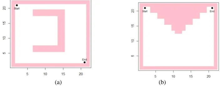
Figure 1. Environment maps.

[image:2.595.119.475.400.545.2]

To illustrate the shortcomings of ant colony algorithm in obstacle avoidance, we take two static environment maps in Figure 1 as examples to simulate ant colony algorithm. In the map, the shadow part is the obstacle area, “Start” represents the starting point, and “End” represents the target node.Then the environment map is discretized into a gray matrix according to 20 *20, where the blank area is the feasible area, and the pink point represents the obstacle area, as shown in Figure 2.

(a) (b)

Figure 2. Gray matrix of environment map.

[image:3.595.124.470.74.217.2]

(a) (b)

Figure 3. Optimal path of traditional ant colony algorithms.

In addition, concave obstacles are set up in the environmental map 1a, which makes the ant colony algorithm easily fall into the local optimal solution. Selecting the trajectory of some single ants, as shown in Figure 4, we can see that the single ant stayed in the concave area for a long time. Using "ant lost" to measure the invalid path, if a single ant fails to reach the target node after 1000 times of transfers or returns to the starting point after many times of transfers, it is recorded as "ant lost". The single ant in Figure 5 returned to the starting point after 658 moves, and the path planning failed.

[image:3.595.128.470.341.494.2]

(a) (b)

Figure 4. The trajectory of single ant.

Finally, the proportion of ants lost is analyzed, and the results are shown in Figure 6 (total number of simulation: 50), from which we can see that the concave area caused a lot of "ants lost". In real UAV path planning, this means that a large number of UAVs can not reach the target node, which not only wastes equipment (UAVs can not reach the target node means that equipment is lost), but also makes the path planning fail.

[image:3.595.291.487.586.722.2] [image:3.595.108.264.589.719.2]

Cellular Ant Colony Algorithm Using Bayesian Posterior Probability

As mentioned above, by gridding the map environment with environmental modeling, the gray scale matrix is obtained. According to the flight characteristics of UAV, obstacle area and feasible area are determined, and each point on the gray matrix corresponds to the environment map one by one. The feasible points are represented by 1, while the infeasible ones are represented by 0 (for details, see Figure 2). At the same time, in order to describe the trajectory of a single ant, its cellular model(represented by Model) is established and briefly described as follow

Model=( , , , )S L N F , (1)

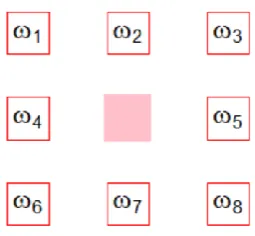
where S denotes cellular state. S i j_n( , ) 1 denotes that a single ant is at a node ( , )i j after n times of transfers. L represents all possible locational nodes arrived by a single ant, i.e. cellular space. N represents the cellular neighborhood, usually expressed by N S( )_n , which represents that, combined with the flight characteristics of UAV, the location nodes that may be reached after n 1

times of movement, as shown in Figure 7. Let i be the direction number and define

( _n) { |_i 1, 2, ,8}

N S  s i , (2)

where s₃ 1 means that a single ant chooses direction ₃ at the (n 1)-transfer, otherwise, if

3 0

[image:4.595.232.360.358.476.2]

s , the direction ₃ is not selected.

Figure 7. Moore cellular neighbor model.

For convenience of discussion, the position of UAV after n times of transfers is represented by

( , )i j , which is usually recorded as ( )n ( , )i j . Cellular Ant Colony Algorithm (CAA) is to determine a transformation function F combined with cusp optimization strategy to select the next coordinate (n 1) in the cell neighborhood, that is,

(n 1) F( ( ))n . (3) Next, Bayesian analysis of ant colony algorithm is carried out.

Firstly, the Bayesian prior probability is determined.

In the new cell neighbor N S₀( _{n 1}), the probabilities of candidate nodes calculated from pheromone matrix are used as the prior probabilities for path selection as follow

0( n)

k k

i i N S

p 









, (4) where _k is the pheromone of the k-th node in the cell neighbor N S₀( _{n 1}).

Secondly, the conditional probability of alternative nodes in cellular neighborhood N S₀( _{n 1}) is determined.

node W_i in the cell neighbor N S₀( _{n 1}),

( i) {dot | ( i, dot) , Angle( ) 100 , dot }

RD W  dist W RR n   L . (5)

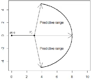
[image:5.595.220.375.172.306.2]

Here, Angle( )n denotes the angle between ( )n , W_iand dot, which indicates that the selection of dot is limited to the sector area with the predicted distance not exceeding RR and the angle between dot and vector ( ),n Wi not exceeding 80 degrees, as shown in Figure 8.

Figure 8. Prediction area of alternative nodes.

The construction of conditional probability of alternative nodes includes three factors: 1. the gravitational field of the target node which is inversely proportional to the distance from the UAV to the target node; 2. the number and importance of obstacle nodes in the fixed area of the UAV; 3. the distance between the UAV and the obstacle node.

According to the gravitational field of the target node, the heuristic function is constructed as follow 1 1 ( ) ( , ) i i f W

dist W End

 ,WiN S0( n1). (6)

Here, the larger f W₁( )_i is, the closer W_i is to the target node.

According to the number and importance of obstacle nodes in fixed area (predicted area) of UAV, the conditional probability can be written as

2

1 ( ) 0,

( ) 1

, Num( )

i

i

i

if Num W f W else W       

, WiN S₀( n₁), (7)

where Num( )W_i denotes the number of obstacle nodes in the prediction area. The more Num( )W_i ,

the smaller the conditional probability f W₂( )_i . Usually, in order to prevent the failure of obstacle

avoidance, UAV needs a certain flight safety distance, which is set as D₀. Considering the distance between UAV and obstacle node, the conditional probability is defined as follow

3 0 0

0

1 ( ) 0,

( ) min{ ( , obstacle) ,1} ( , obstacle) , 0 ( , obstacle) ,

i

i i i

i

if Num W

f W dist W D dist W D

dist W D

       _ 

, (8)

where the smaller the minimum distance mindist W( , obstacle)_i between node W_i and obstacle is,

the smaller the conditional probability f W₃( )_i is. The importance of heuristic information of target node, the importance of obstacle distribution (the number of nodes in predicted area), and the importance of minimum distance between UAV and obstacle node are respectively expressed by ₁,

1 1 2 2 3 3

( )_i ( )_i ( )_i ( )_i

f W f W f W f W , (9)

where ₃ 1 _{1 2}, ₁ 0, ₂ 0, ₃ 0. Then the conditional probability of the candidate nodes can be obtained by normalization as follow

0( 1)

( ) ( ( ) ) ( ) i n i i i W N S

f W

P n W

f W











. (10) Thirdly, the posterior probability of the candidate nodes in cell neighbor N S₀( _{n 1}) is determined. According to Bayesian formula, the expression of posterior probability is

0( 1)

( ) ( ( ) ) ( ( )) ( ) ( ( ) ) i n i i i i i

W N S

P W P n W

P W n

P W P n W

     



, (11) where P W( _i ( ))n is a posterior probability obtained by Bayesian decision, which is used to decide

candidate nodes. In the Moore Cellular Neighbor Model, the moving direction k is selected to make

1 2 8

max{ ( ( )), ( ( )), , ( ( ))} k

p  P W  n P W  n P W  n , (12) where1 k 8. This completes the one-time transfer of a single ant.

Finally, the pheromone of UAV is updated. If the k-th node (n 1) of the cell neighbor

0( n 1)

N S is selected according to the probability p_k in the optimized trajectory, then the pheromone of the k-th node is updated by the following local update rule

(1 )

k r k r k

      , (13) where r is a constant, representing the Volatilization Coefficient of information. Suppose that the k-th node of cell neighbor N S₀( _{n 1}) is (n 1), then

( ( ), ( 1))

k

Q

d n n , (14)

where d( ( ), (n n 1)) represents the distance between node ( )n and node (n 1).

Based on the above, the steps of Bayesian cellular ant colony algorithm based on posterior probability are shown as follows:

(1) The map is discretized and the gray matrix is established.

(2) Set the number of flight simulations to n and the number of unmanned aerial vehicles to m.

(3) Set the pheromone matrix IM, whose dimension is the same as the gray matrix H, and all the elements are valued at 1.

(4) The cycle of the number of flights begins with for（i 1 :n）. (5) The cycle of the number of aircraft begins with for（j 1 :m）. (6) The while loop (or repeat) starts until the target node is found to stop.

(7) Assuming that the position of the j-th UAV in the i-th cycle is Poisition (i, j), the feasible region in its cell neighborhood is determined by gray matrix.

(8) Cusp optimization is carried out to eliminate the nodes that do not conform to the flight angle in the feasible area to determine the alternative nodes.

(9) Determining the prior probability of each candidate node Wi according to pheromone.

(10) The conditional probability and posterior probability of the candidate node Wi in the prediction region are calculated in turn.

(13) At the end of the number cycle of aircraft, m paths are determined, and the optimal path for this simulation is selected according to the shortest distance.

(14) The pheromone is updated according to the optimal trajectory and Q m,r 0.05.

(15) The cycle of the number of flights is over, and the optimal path is selected by synthesizing the results of N flight simulation.

Simulation

In order to verify the correctness and validity of the proposed algorithm, 300 unmanned aerial vehicles are used for calculation (30 units per round, 10 rounds of continuous transmission, updating the pheromone matrix of the next round based on the flight results of the previous round). In the same environment as Figure 1, Figure 1(a) sets the initial position as (1,21), the target node as (21,1), Figure 1(b) sets the initial position as (1,21) and the target node as (21,21). The Volatilization Coefficient r 0.05 was chosen. In Bayesian cellular ant colony algorithm based on posterior probability,

1 2 3

1 3

    . (15)

Note that the environmental map is discretized according to20 20 , and the radius of the predicted area is RR 3.

Firstly, the optimal path problem is considered, and the simulation results of the traditional ant colony algorithm (see Figure 3 and Figure 4) and the improved Bayesian ant colony algorithm (see Figure 9) are compared. It can be seen that the new ant colony algorithm has enhanced obstacle avoidance ability and improved the shortcomings of trapping in concave area after incorporating Bayesian strategy.

[image:7.595.113.481.418.564.2]

(a) (b)

Figure 9. Simulation results based on posterior probability ant colony algorithm.

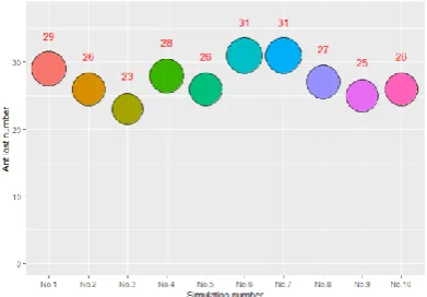
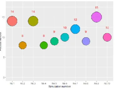
Figure 10. Ant lost number based on posterior probability ant colony algorithm.

[image:7.595.208.392.590.732.2]

after introducing Bayesian ant colony algorithm, the phenomenon of ants lost is significantly reduced.

Summary

In the global static environment, aiming at the shortcomings of traditional ant colony algorithm in obstacle avoidance and path planning in concave area, an improved Bayesian ant colony algorithm based on posterior probability is proposed. The algorithm takes grid map as environment map, and integrates the Heuristic information of target nodes and repulsive information of obstacles into conditional probability in the search process of ant colony algorithm.Then the posterior probability is calculated as the Bayesian path selection probability, which increases the obstacle avoidance ability of UAV and alleviates the shortage of easily trapping in concave area.The simulation results show that the improved algorithm can find the optimal path more effectively.

Acknowledgement

This research was financially supported by the Guizhou Science and Technology Plan Project ([2016]7081).

References

[1] X.F. Wang, S.Y. Yang, Dynamic path planning of UAV based on cellular ant colony algorithm, Machinery & Electronics, 36 (2018) 69-72.

[2] Y.Y. Zhang, Z. Zhang, Q. Wang, Robot path planning based on improved multi-step ant colony algorithm, Computer Engineering And Design, 39(2018) 3829-3834+3866.

[3] M.F. Luo, A Research on Unman Aerial Vehicle 3D Path Planning using Probabilistic Roadmap Method, Huazhong University of Science & Technology, 2016.

[4] S.Y. Yang, Y.Y. Liu, W.L. Yang, A Local Dynamic Probabilistic Roadmap Method for Unknown Environment, Aeronautical Science & Technology, 27(2016) 69-73.

[5] Z.K. Zhou, A Research and Simulation of Mobile Robot Path Planning Combined with Artificial Potential Field and Ant Colony Algorithm, China's Manganese Industry, 36(2018) 182-187.

[6] X.Y. Wang, L. Yang, Y. Zhang, S. Meng, Robot path planning based on improved ant colony algorithm with potential field heuristic, Control and Decision, 33(2018) 1775-1781.

[7] J.X. Liu, Y.K. Zhao, Path planning of cellular Bayesian decision, Computer Engineering and Design, 30 (2009) 4053-4056.