F 2018 IX International Conference on Optimization and Applications (OPTIMA2018)
ISBN: 978-1-60595-587-2
On
Existence
of
Optimal
Non-destructive
Controls
for
Ecosystem
Exploitation
Problem
Applied
to
a
Generalization
of
Leslie
Model
Alexander
SMIRNOV
∗and
Vladimir
MAZUROV
KrasovskiiInstituteofMathematicsandMechanicsUBRAS,Ekaterinburg,Russia
∗ Correspondingauthor
Keywords: Concaveprogramming,Managingofrenewableresources,Non-destructiveexploitationof ecosystems,NonlinearLesliemodel.
Abstract. We proposedearlier somegeneral formalizationfor the problem of the nondestructive
use of renewable resources and reduced it to some mathematical programming problem. In this
article,we studysomepropertiesof optimalcontrolsfor thismathematical programming problem
in the particular case of obtained earlier by authors nonlinear generalization of so-called Leslie
model. We establishthe existence of optimalcontrols that preserve the structure of the operated
system, assuming the concavity of the functions used. It turns out that there existsa hyperplane
containing such controls. We use some generalization of the classical concept of irreducibility
for nonlinear maps, the concept of local irreducibility. These results have applications to actual
problems of rational exploitation of naturalresources.
Introduction
First we introduce a basic notation. Let Rq+ be anon-negative orthant of Rq which inducesa
standard partial ordering: we write x ≤y if y−x∈ Rq+, x<y if y−x ∈intRq+, where intM is
the interiorofasetM. Wealso writex yifx≤y andx6=y. Next,Zmeansthe setof integers;
m,n = {i ∈ Z | m ≤ i ≤ n}. For brevity sake, x = (x1,x2,...,xq) will sometimes be written
as x = (xi). The iteratives of a map F are denoted by Ft(x) (t = 1,2,...), F0(x) ≡ x. Sets of
nonzerofixed pointsand positive fixedpoints of F are denoted by NF and N+, respectively.
We study here some formalization for the problem of sustainable exploitation of ecological populations. The basic concerns taken into account include management of fisheries, agriculture, forestry, and other renewable resources, including harvesting of wildlife mammals populations. This problem is highly relevant at the present time since often commercial overexploitation of populations occurs. This leads to an unbearable burden on regulatory mechanisms of the restora-tion of popularestora-tions, and as a result, their degradarestora-tion. So, according to the UN, about a third of the stocks in marine fishing are registered as caught [1]. The reduction in forest area (by about 1% over the past 25 years) is one of the leading causes of climate change.
The problem of sustainable exploitation of ecological populations is characterized by an abun-dance of diverse approaches to the understanding of feasible and optimal impacts (controls) for various specific natural systems (see, for example, the review in [7]). Note that the removal of a part of the population can seriously affect its behavior, genetic composition, etc., i.e. is a way to manage the population and its units. Therefore, we will continue to talk about the management of the population on the basis of control actions (controls).
Most research in this area includes the use of specific models to find the maximum allowable exploitation of commercial populations. Early theoretical studies in this direction were devoted to the search for correct mathematical settings of resource management problems and their analysis. To solve the problem of maximum permissible removal of individuals from structured populations, matrix models were used, when the transition to a next state is carried out using a matrix called the population projection matrix [3]. The population structure was usually identified with the structure of an eigenvector corresponding to the dominant eigenvalue of this matrix. Analytical studies of these strategies were later carried out in [5], where some concepts natural for the exploitation of ecosystems were formalized, and the corresponding statements were rigorously proved. It was in this article that the relationship between the optimal exploitation of populations and the solution of problems of mathematical programming was clearly formulated for the first time.
The approach to optimal exploitation, based on the stationary structure of the population, has long been prevalent; while the concept of sustainable exploitation was variously determined by different authors. The exact mathematical formulation of the problem varied among different authors, depending on the needs of practical applications in specific problems. One of the first theoretical studies in this direction was the article [6]. Here the concept of sustainable exploitation (SY — Sustainable Yield) was defined, and the solvability of the corresponding optimization problem was formulated and proved. Later a more general problem of the finding of the maximum balanced (permissible, stable) level of exploitation was called the Maximum Sustainable Yield problem (MSY-problem) [7]. The concept of MSY is still one of the cornerstones of managing renewable resources [4].
The first successful attempts to take into account nonlinear connections considered a nonlinear dependence on population density only for the first age class [18]. Later in [9] was considered a model with the dependence of reproductive and survival rates on density for all age classes. In all the above studies, optimal strategies were sought for an equilibrium structure of the population. They used multiplicative control, that is, they sought out fractions of age groups that could be seized without causing irreversible damage to the population.
A detailed review of the economic aspects of the problem of the rational use of renewable resources can be found in [4]. This line of research (initially developed for commercial fishing) explicitly takes into account the organizational and economic costs, the so-called harvesting effort. Early work in this area took into account only the general biomass of the population — model of excess production of Gordon and Schaefer (other names — biomass model or surplus-model). Later work took into account the age structure of the population (for details and references, see [21]).
We consistently develop here a general approach to the formalization of the population exploita-tion problem, proposed in [14]. Our model does not attempt to cover the entire scale complexity of the problem in an abundance of details of the available links and numerous parameters. The necessity of constructing and studying such models (usually called compact or global ones) is em-phasized in [4]. Models of this kind with the properties studied should serve as a basis for creating more detailed models of specific natural systems. The basic properties of detailed concrete models follow from the corresponding properties of basic global models.
The purpose of this paper is to study the properties of the feasible set of problem (4) in the case when the ecosystem is described by some nonlinear generalization of so-called Leslie model.
The Leslie model refers to models of projection type. This model is described by iterative
process (1) with the matrix
L=
f1 f2 . . . fn−1 fn s1 0 . . . 0 0
0 s2 . . . 0 0
..
. ... . . . ... ... 0 0 . . . sn−1 0
,
also called the Leslie matrix, as the step operator. The Leslie model allows to describe discrete age- and, more generally, stage-structured populations. This model is widely used by ecologists to study global dynamics of an age distribution of natural biological populations.
Here, fi and si are the fertility and survival rates in age groups. We leave aside biological
assumptions adopted in a derivation of this model and in general, biological aspects associated with this model; a detailed discussion of these questions can be found in [3].
The Leslie model is one of the most common models in studies of natural ecosystems since its relationships are a natural consequence of natural assumptions about the interaction of age groups. The properties of this model are well studied (see, for example, [12]). Further development of the Leslie model occurred by easing its limitations and developed mainly in two directions. Within the framework of the first direction, the transition from the age structure to the more general stage structure was carried out; the second direction was associated with the consideration of the additional (status) structure, and, thus, with the transition to the binary structure of the population.
Apparently, for the first time the idea of classification not by age, but by some other, more easily observed or measurable characteristics was realized in [11]. Here it was proposed to use as a basis for classification the successive stages of the development of the organism (different, generally speaking, duration). Alternative signs of classification were also examined in [22] — instead of age, the size of trees was taken into account when modeling forest populations.
More adequate account of the structure of the population is associated with both a transi-tion from the age to the stage structure and with the introductransi-tion of additransi-tional features of the population partition. Additional signs of classification, in addition to age and size, can be, for example, such characteristics as volume, biomass, genotype (phenotype), physiological parameters of individuals, etc. The movement along the life cycle in such models also reflects the parallel transitions between the groups of this additional structure. This additional structure is called the status structure. The notion of a generalized stage of development of individuals is formed as the basis for their classification [3]. The classification of individuals in such models turned out to be ”two-dimensional”: the state of a population is more conveniently described not by a vector, but by a certain matrix. One of the earliest such publications is the article [23], which took into account the breakdown into genotypes.
In [8] it was proposed to classify individuals not only by age but also by the number of repro-ductive acts. Here, for the first time, a generalization of the Leslie matrix appeared, in which the matrix-blocks replace the elements of the Leslie matrix.
The binary structure was used in [10] to model the dynamics of a plant population. Since their flowering begins only after reaching a certain size, this model together with the age of the plants also took into account their size.
A detailed review of the properties of above generalizations of the Leslie model can be found in [13].
One of the early models that took into account the two-dimensional (binary) structure of the population was proposed in the middle of the seventies of the last century in [2]. In this article, a subdivision of a certain natural population was modeled according to an additional feature (genotype), in addition to age. This model was generalized in [19], where dynamic properties of some general class of nonlinear dynamical systems were investigated. It is this generalization that will be used by us further in the problem of optimal exploitation of the population. This model will be described in more detail below.
Some Preliminary Results
Our general approach to this problem regards the ecosystem as a discrete dynamical system of the form
xt+1 =F(xt), t = 0,1,2, . . . , (1)
where xt means a system state at time t = 0,1,2, . . ., a step operator F transforms the system
from the previous state to the following. Based on the biological interpretation, it is necessary to
assume that this system has a trivial equilibrium state: F(0) = 0.
An operated system is modeled by the iterative process
xt+1 =Fu(xt), t= 0,1,2, . . . , (2)
where x = (xi), u = (ui), Fu(x) = (F(x)− u))+, a+ = max{a,0}, x+ = (x+i ). We write
{xt(x0, u)}+t=0∞, xt(x0, u) = (xit(x0, u)) for the realization of (2) with the initial vector x0. In [14]
we formulated an optimization problem for dynamical system (1): is to be found
˜
c= max{c(u)|u∈U}, (3)
where c(u) is the total effect of using of u, and the feasible set U is the closure of the set
U ={u∈Rq+ |X0(u)6=∅}
of controls. The control vector u is feasible if and only if there exists an initial statex0 such that
the system (2) stably exists for an indefinitely long time:
X0(u) = {x0 ∈Rq+|inf
t x i
t(x0, u)>0 (∀i∈1, q)}
Thus the set U formalizes the requirement of the indestructability of the managed object. We
showed that problem (3) is equivalent to the following mathematical programming problem:
max{c(u)|x=F(x)−u, x≥0, u≥0} (4)
So, ˜c, ˜u is a solution of problem (3) if and only if ˜c, ˜u, ˜x is a solution of problem (4). The
following assumptions were used: the map F was assumed to be nonnegative and concave on Rq+
(and hence monotone increasing on Rq+), the function c(u) was assumed to be nonnegative and
monotone increasing. Also a natural condition for an absence of identically zero coordinates of
F(x) = (fi(x)) was satisfied:
∀i∈1, q ∃x∈Rq+: fi(x)>0. (5)
From these assumptions follows that F(intRq+)⊆intRq+.
We also use a local analogue of a classical concept of irreducibility [17] of a map, the property of irreducibility at some point. In particular, the concept of irreducibility at zero turned out to be especially useful. For the corresponding definitions we introduce the following sets:
I+(x) ={i∈1, q|xi >0}, I0(x) = {i∈1, q|xi = 0}.
A map F ∈ {Rq+ 7→Rq+} is said to be reducible at point y = 0 (reducible at zero), if
∃x∈Rq+: x0, I0(x)6=∅, I0(x)⊆I0(F(x)).
Properties of the local irreducibility are studied in [15]. Among other things, the irreducibility of a map at zero guarantees the positiveness its non-zero fixed points.
It is clear that a necessary condition for the possibility of exploitation of a population is its stable existence in the absence of control, i.e. the presence of a non-trivial equilibrium of
the iterative process (1). We now formulate a sufficient condition for NF 6= ∅ in the class of
concave dynamical systems. We assume that the map F is defined on the whole Rq+; therefore
this map is also monotone increasing. For such map we can define positively homogeneous maps
Fs(x) = lim
α→+sα
−1F(αx) (s ∈ {0,∞}) with F
∞(x) ≤ F(x) ≤ F0(x) (∀x ∈ R
q
+). There is a
well-developed spectral theory of positively homogeneous maps; in particular, the notion of the
dominant eigenvalue λ(H) of the map H that has many properties of the corresponding concept
for matrices can be defined [17]. It is not difficult to verify that the condition
λ(F∞)<1< λ(F0). (6)
is sufficient for the existence of a nonzero fixed point of the concave map F.
It was shown in [14] that then the set NF is bounded, convex and contains the largest element
¯
xF. If F is also irreducible at zero, then set U contains some positive vector, is also convex and
downward, because with each positive vector ualso contains the whole segment [0, u]. Besides the
following equalities hold:
U ={u∈Rq+ |Nu+6=∅}, U ={u∈Rq+|Nu 6=∅}, (7)
where by Nu and Nu+ we denote the sets of nonzero fixed points and positive fixed points of Fu,
respectively.
We introduce a set
D={u∈Rq+|Nu 6=∅, Nv =∅(∀v > u)} (8)
that forms a part of the boundary of U. The set Dcontains all potentially optimal vectors of the
problem (3). We divide this set into two disjoint parts by criterion of the presence or absence of
common points with U:
D0 =D\D00, D00=U \U. (9)
From equalities (7), (9) we obtain the following representation of D00:
D00 ={u∈Rq+ |Nu 6=∅, Nu+ =∅}. (10) Directly from (8)–(10) the following representation follows:
D0 ={u|Nu+6=∅, Nv =∅(∀v > u)}. (11)
In [16], the properties of D0, D00 were analyzed in terms of the dominant eigenvalues of some positively homogeneous maps.
Let us turn to the above generalization of the Leslie model [19]. Thus, there arem≥1
intrapop-ulation structural units (subdivisions), each of which contains individuals ofnages 1,2, . . . , n. Let
x(i,jt) denote the number of individuals of subdivision i∈1, m of age j ∈1, n at time t = 0,1,2. . .,
then the model under consideration have the following form:
x(i,t1+1) =fi(at), x(i,jt+1)+1 =αi,jx(i,jt) (i∈1, m, j ∈1, n−1). (12)
Here αi,j > 0 and βi,j ≥ 0 are the survival and fertility rates in the structural population units,
at = Pmi=1Pnj=1βi,jx(i,jt) — the total number of joung in population at time t. Denote π
(i)
j =
Qj−1
`=1αi,` (by convention
Qs
`=ra` = 1 for r > s), we obtain the system of equations for finding an
equilibrium of (12):
xi,j =π
(i)
j fi(a(x)) (i∈1, m, j ∈1, n), a(x) =
m
X
i=1
n
X
j=1
βi,jxi,j. (13)
As we see from (13), for the model (12) any nontrivial equilibrium state is always positive even without the assumption of irreducibility. Using the lexicographic order for the numbering of coor-dinates, we obtain the population state vectorx= (x(1), x(2), . . . , x(m)), wherex(i)= (xi,1, . . . , xi,n),
i∈1, m, which is transformed into the next state by the following step operator F(x) = (fi,j(x)):
fi,1(x) =fi(a(x)), fi,j+1(x) =αi,jxi,j (i∈1, m, j ∈1, n−1). (14)
This map is concave if the following condition is satisfied:
fi(a) are concave onR+ (∀i∈1, m). (15)
Condition F(0) = 0 means that fi(0) = 0 (∀i ∈ 1, m); from (5) it follows that all functions fi(a)
are positive for a >0. Thus the following property is satisfied:
fi(0) = 0, a >0⇒fi(a)>0 (∀i∈1, m). (16)
The maps F0, F∞, which determine the existence of a non-trivial equilibrium state of (12), are
linear and have the following components:
fsi,1(x) = fi0(+s) m
X
i=1
n
X
j=1
βi,jxi,j, fsi,j+1(x) = αi,jxi,j (i∈1, m, j ∈1, n−1),
wherefi0(+s) = lim
α→+sα −1f
i(α) (s = 0,∞; i∈1, m) is the right-hand derivative offi(a) at zero (for
F0) or, respectively, the derivative of this function at infinity (forF∞). The structure of matrices
L0, L∞ defining these maps coincides with the structure of a nonnegative mn×mn matrix Lmn ,
which is a generalization of the Leslie matrix. In general, it has the following entries:
li,j =
apr,t, i= (p−1)n+ 1, j = (r−1)n+t(t ∈1, n),
br−p 1, i= (p−1)n+r, r ∈2, n, j =i−1,
the rest of entries are zero. For example, for m= 2, n = 3 this matrix has the following form:
L23 =
a(1)1,1 a(1)1,2 a(1)1,3 a(1)2,1 a(1)2,2 a(1)2,3 b(1)1 0 0 0 0 0
0 b(1)2 0 0 0 0
a(2)1,1 a(2)1,2 a(2)1,3 a(2)2,1 a(2)2,2 a(2)2,3
0 0 0 b(2)1 0 0
0 0 0 0 b(2)2 0
.
In the case of the model (12) a(r,tp) = fp0(+s)βp,t, b
(p)
r−1 = αp,r−1 (p ∈ 1, m, r ∈ 2, n, t ∈ 1, n).
According to results of [20], sgn(λ(Ls)−1) = sgn(σ0(+s)−1), where
σ(a) = m
X
i=1
σ(i)fi(a), σ(i)=σin, σji = j
X
k=1
βi,k k−1
Y
`=1
αi,` (i∈1, m, j ∈0, n). (17)
Here sgn(x) =|x|/x for x6= 0, and sgn(0) = 0. Thus, (6) can be rewritten in the form
σ0(+∞)<1< σ0(+0), (18)
Here σ(a) is nonnegative, monotone increasing, and concave. The condition (18) means the
solv-ability of equation σ(a) = a. Its unique positive solution ¯aF corresponds to the unique positive
fixed point ¯xF of the map (14): ¯aF =a(¯xF).
By [15], the irreducibility at zero of concave on Rq+ mapF is equivalent to the irreducibility at
zero of F0, and the matrix Lmn for model (14) is irreducible if and only if the condition
βi,n>0 (∀i∈1, m) (19)
holds [20]. So, (19) is a necessary and sufficient condition for irreducibility at zero of the map (14).
Properties of Optimal Controls of the Optimal Harvesting Problem for the General-ized Leslie Model
The feasible set U for the model (12) in addition to the restrictions of nonnegativity of x,u is
given by equations
xi,1 =fi(a(x))−ui,1, xi,j+1 =αi,jxi,j−ui,j+1 (i∈1, m, j ∈1, n−1), (20)
where a(x) =
m
P
i=1
n
P
j=1
βi,jxi,j. Recall that xi,j means the number of individuals of subdivision i of
age j, ui,j means the number of individuals of age j removed from subdivisioni in an equilibrium
state of the system (2) for the map (14).
We need the following notation (further i∈1, m, j, k ∈1, n):
π(i)=π(ni), πj(i) =p(1i,j), pj(i)=p(j,ni), p(≤ji) =p(1i,j), p(j,ki) = k−1
Y
`=j
αi,`, (21)
qj(i) =qj,n(i), qj,k(i) = k
X
s=j βi,s
s−1
Y
t=j
αi,t (i∈1, m, j, k ∈1, n), (22)
p(i)(u) = n
X
j=1
p(ji)ui,j, p
(i)
≤(u) =
n
X
j=1
p(≤ji)ui,j q(u) = m
X
i=1
n
X
j=1
qj(i)ui,j, (23)
µ(a) = σ(a)−a, λi(a) = π(i)fi(a) (i∈1, m). (24)
Note that because ofσ(0) = 0 and σ(¯aF) = ¯aF, we have µ(0) =µ(¯aF) = 0.
It is not difficult to find an explicit expression for coordinates of x(i):
xi,j =π
(i)
j fi(a)−p
(i)
≤j(u) (j ∈1, n−1), xi,n=λi(a)−p(i)(u) (∀i∈1, m). (25)
Nonnegative x, u satisfying these equations are feasible if a = a(x). In this case we write the
vector x with coordinates (25) as x = x(a, u), explicitly indicating a and u that give x. Note
that the nonnegativity (positivity) of the last coordinate of x(i) is equivalent to the nonnegativity
(positivity) of all its coordinates:
xi,n≥0⇒xi,j ≥0, xi,n >0⇒xi,j >0 (∀i∈1, m, j ∈1, n). (26)
The variable a, which in this system of constraints can be considered as a parameter, belongs
to the set A={a≥0| ∃u≥0 :x=x(a, u)≥0}. Obviously, the largest element of this set is ¯aF.
Multiplying equalities (25) by βi,j and summing, we get the equation
q(u) = µ(a). (27)
Thus, ifxu ∈Nu, then (27) holds, which for a givenu can be regarded as an equation with respect
to a.
From (25) and (26), we derive the following parametric representation of U:
U ={u| ∃a∈[0,a¯F] : pi(u)≤λi(a) (∀i∈1, m), q(u) = µ(a), u≥0}. (28)
A similar representation holds also for U, with the strict first inequality in (28) instead of the
nonstrict one.
It follows from (18) that 0 < µ∗ = max
a≥0 µ(a) < +∞ and A
∗ = Argmax
a≥0 µ(a)6=∅. Denote
a∗ = minA∗, a∗ = maxA∗. By definition of µ∗, the equation (27) yields
q(u)≤µ∗ (∀u∈U). (29)
Clearly, the functionµ(a) is nonnegative and concave on [0,¯aF]. We give some other properties of
this function, which will be needed in the sequel.
Lemma 1.Suppose that conditions (15)–(16), (18) are satisfied. Then the following assertions hold:
(i) µ(a) is strictly increasing on [0, a∗], is constant on [a∗, a∗] (ifa∗ < a∗), and is strictly decreas-ing on [a∗,¯aF].
(ii) If µ ∈ (0, µ∗) then equation µ(a) = µ has exactly two solutions a1, a2 with 0 < a1 < a∗ ≤
a∗ < a2 <¯aF.
Let Γ be a nonnegative part of the hyperplane q(u) =µ∗:
Γ ={u∈Rq+ | q(u) = µ∗}.
Recall that D0 denotes the closure of D0. The following statement shows that the
structure-preserving controls form a part of the hyperplane.
Theorem 1. Suppose that conditions (15)–(16), (18)– (19) are satisfied. Then the following equalities hold:
D0 = Γ∩U, D00∩Γ⊂D0, D0 = Γ∩D. (30)
Proof. Let us prove the first of these equalities. Representations (7), (11) yield D0 ⊂ U; we now
show that D0 ⊂Γ.
Letu∈D0, and assume, by contradiction, thatu /∈Γ. Then it follows from (29) thatq(u)< µ∗.
Therefore, by statement (ii) of Lemma 1, equation (27) has exactly two solutions a1, a2 with
0 < a1 < a∗ ≤ a∗ < a2. Obviously, a(¯xu) = a2. By (7), (25) from u ∈ U we get ¯xi,n(u) =
λi(a2)− p(i)(u) > 0 (∀i ∈ 1, m). We show that the assumption u /∈ Γ implies an existence of
u0 with u0 > u also belonging to U. Take any such that 0 < < x¯i,n(u) (∀i ∈ 1, m). Let u0 =u+u(δ), where u(δ) is a vector whose coordinates are all δ >0. Denoting
p(0i)= n
X
j=1
p(ji) (i∈1, m), q0 =
m
X
i=1
n
X
j=1
q(ji),
we get from (21)–(23) equalities
p(i)(u0)−p(i)(u) = p(i)(u(δ)) =p(0i)δ, q(u0)−q(u) = q(u(δ)) =q0δ. (31)
The second of these equalities shows that, in addition to the inequality q(u) < µ∗, the inequality
q(u0)< µ∗ also holds for 0< δ < δ0, whereδ0 = (q0)−1(µ∗−q(u)).
By Lemma 1, there exists a function h(µ) inverse to the function µ(a) on [a∗,¯aF]. Because
a0 = h(q(u0)) satisfies the equation µ(a0) = q(u0), it follows from (28) that a0, u0, ¯xu0 = x(a0, u0)
satisfy the system (20). In particular, denoting ¯xu0 = (¯xi,j(u0)), we get from (25): ¯xi,n(u0) =
λi(a0)−p(i)(u0) (∀i∈1, m). To complete the verification of the condition u0 ∈ U, it remains to
show that p(i)(u0)< λ
i(a0), or, what is the same, ¯xi,n(u0)>0 (∀i∈1, m).
The map ¯x(u) : u → x¯u is strongly decreasing (see [14, Lemma 1(6)]), hence ¯x(u) > x(u¯ 0),
so 0 < x¯i,n(u)− x¯i,n(u0) = (λi(a2)−λi(a0)) + (p(i)(u0)− p(i)(u)). Because of continuity of the
superposition of continuous functionsλi(a) anda=h(q(u)), there exists a sufficiently smallδ1 >0
such that 0 < λi(a2)−λi(a0) < ε/2 for 0 < δ < δ1. Further, from the first equality in (31)
it follows that 0 < p(i)(u) − p(i)(u0) < ε/2 (∀i ∈ 1, m) for 0 < δ < δ2, where δ2 = ε/2p0,
p0 = max{p
(i)
0 : i ∈ 1, q}. Therefore, for u0 = u +u(δ) with 0 < δ < min{δ0, δ1, δ2} we get
0 < x¯i,n(u)−x¯i,n(u0) < ε (∀i ∈ 1, m). Hence ¯xi,n(u0) > x¯i,n(u)−ε > 0, because of our choice ε >0. Therefore ¯x(u0) = x(a0, u0) >0 and, in view of (7), u0 ∈ U. But this, by (11), contradicts
the condition u∈D0, because of u0 > u. Thus, the assumption u /∈Γ led to a contradiction. This
means that u /∈Γ, and, consequently, u∈Γ∩U. The property D0 ⊆Γ∩U is proved.
Conversely, if u ∈ U and u ∈ Γ then, by (7), N+
u 6= ∅. Further, from (19) we get q
(i)
j =
Pn
k=jβi,k
Qk−1
`=j αi,` ≥βi,n
Qn−1
`=j αi,` >0, therefore, q(v)> q(u) =µ
∗ for v > u. But then it follows
from (29) that Nv = ∅ (∀v > u); by (11) this implies u ∈ D0. The property Γ∩U ⊆ D0 is also
proved, and, thus, the first equality in (30) is completely proved.
Let us prove the second equality in (30). We choose some point u ∈ D00 ∩Γ and define a
sequence uk= (1−αk)u+αku0, where u0 ∈D0 ⊆Γ, αk∈(0,1) andαk→0 as k →+∞. Clearly,
uk → u as k → +∞. From (11), by u0 ∈ D0, it follows that ¯xu0 > 0. The map ¯x(u) is concave,
therefore, ¯xuk ≥(1−αk)¯xu+αkx¯u0 ≥αkx¯u0 >0, that is, ¯xuk >0, so ¯xuk ∈N +
uk. Because of u∈Γ
and u0 ∈Γ, we get uk ∈Γ, so that q(uk) =µ∗ (k= 1,2, . . .).
If v > uk, thenq(v)> q(uk) =µ∗ and, because of (29),Nv =∅. But, by (11), this means that
uk ∈D0. Thus, the point u is indeed the limit point of D0.
It remains to prove the last equality in (30). We first prove the inclusionD0 ⊆Γ∩D. It follows
from D0 ⊆D, D0 ⊆Γ that D0 ⊆Γ∩D. We now prove this inclusion for limit points of D0. Let u
be a limit point of D0 and uk →u as k →+∞, where uk ∈D0. It follows from uk ∈D0 ⊂ Γ that
N+
uk 6= ∅, so that F(¯xuk)−uk = ¯xuk, and u ∈ Γ. The sequence {x¯uk} is bounded; consequently,
there exists a convergent subsequence of it. For brevity of notation, let it be the sequence {x¯uk}
itself: ¯xuk → x. Then¯ F(¯x)−u = ¯x, so ¯x ∈ Nu and, consequently, Nu 6= ∅. Further, if v > u,
then also v > uk if k is large inaf, hence, Nv = ∅. But this means that u ∈ D. Because it was
previously received that u∈Γ, we get u∈Γ∩D. The inclusion D0 ⊆Γ∩D is proved.
We now prove the inclusion Γ∩D ⊆ D0. Let u ∈ Γ and u∈ D. If u ∈ U, then u∈ Γ∩U =
D0 ⊂ D0, and the checked inclusion is valid. If now u /∈ U, then from (10) because of u ∈ D we
get u ∈ D00, so that u ∈ D00∩Γ. But this implies u ∈ D0 in view of the inclusion D00∩Γ ⊂ D0
proved above. The theorem is completely proved.
We now clarify the representation (28) for the boundary D of U. If u∈U, then we can define
a set
I0(u) ={i∈1, m|x¯i,n(u) = 0}.
Corollary 1. Suppose that conditions (15)–(16), (18)– (19) are satisfied. Then the following assertions hold:
(i) u∈D0 if and only if the following constraints are satisfied:
p(i)(u)< λ∗i (∀i∈1, m), q(u) =µ∗, u≥0; (32)
(ii) u∈D00 if and only if I0 =I0(u)6=∅ and following constraints are satisfied:
p(i)(u) = λi(a) (∀i∈I0), p(i)(u)< λi(a) (∀i /∈I0), q(u) =µ(a), u≥0, (33)
where a= ¯a(u) is the larger root of equation (27).
We now characterize the structure ofD00(in caseD006=∅). Clearly, the function ¯a(u) = a(¯x(u)),
where a(x) is defined by (13), is nonnegative, monotone decreasing and concave on U. Moreover,
¯
a(u) = a∗ (∀u∈D0), and ¯a(u)> a∗ (∀u∈D00\Γ). For a closed set V ⊆U we denote
max{¯a(u)|u∈V}= ¯aV. Note that ¯aU = ¯aF, ¯aD0 =a∗, ¯aD = ¯aD00 for D00 6=∅.
Consider a polyhedron D(a), given by restrictions
p(i)(u)≤λi(a) (∀i∈1, m), q(u) =µ(a), u≥0 (a ∈[0,¯aF]), (34)
where, we recall, ¯aF =a(¯xF). This polyhedron is of interest in connection with the fact that, by (28), the following representation of a feasible set holds:
U =∪{D(a)|a∈[0,¯aF]}. (35)
Not all elements of D(a) belong to D00, therefore we introduce a set
E(a) =D00∩D(a) (a∈[a∗,¯aD]). (36)
Clearly D00 has a representation similar to (35):
D00=∪{E(a)|a∈[a∗,¯aD]}.
Fixa ∈[a∗,¯aD], i∈1, m, and denote
Mi(a) ={u|p(i)(u) =λi(a), p(j)(u)≤λj(a) (∀j 6=i), q(u) = µ(a)}.
By definition (36), E(a) is no longer a polyhedron. Its structure is characterized by following
statement, which follows from Corollary 1.
Corollary 2.Suppose that conditions (15)–(16), (18)–(19) are satisfied. Then the set E(a) is representable in the form
E(a) = ∪m
i=1Li(a) (a∈[a
∗ ,¯aD]),
where Li(a) =Mi(a)∩R+mn, and Mi(a) is an (mn−2)–dimensional affine manifold (∀i∈1, m).
It is not difficult to give examples of models of the form (20) with D00 = ∅. But, as it turns
out, for D0 the situation is quite different. Let us show that the set D0 6=∅ for all models of the
form (20).
We introduce the following notation:
σk(a) =
m
X
i=1
σ(ki)fi(a) (a∈[a∗,a¯D]), σ∗k=σk(a∗). (37)
By definition (17), σ(ki) are monotone increasing with respect to subscript; therefore, the same is
true of σk(a), so that σk+1(a)≥σk(a) (∀k ∈0, n−1).
We also introduce the following sets:
K(a) = {k∈1, n: σk−1(a)< a}, K∗ =K(a∗). (38)
Because σi
0 = 0 (∀i ∈ 1, m), it follows from σ0(a) = 0 that K(a)6= ∅. By monotonicity of σk(a)
with respect to subscript, the following equalities hold:
K(a) = 1, k(a), K∗ = 1, k∗,
where k(a) = maxK(a),k∗ = maxK∗, so k(a)≥1,k∗ ≥1.
For given population state vector x = (x(1), x(2), . . . , x(m)) we collect the positive coordinates
indexes of x(k) = (x
k,1, . . . , xk,n) in the sets Ik+(x):
Ik+(x) ={j ∈1, n: xk,j >0}(k ∈1, m).
We define the sets of vectors u∈Rmn
+ having exactlym positive coordinates that are in the blocks
u(1), u(2), . . . , u(m) of u at the same places:
Uj ={u≥0|Ik+(u) ={j}(∀k ∈1, m)} (j ∈1, n).
The following statement gives a criterion for the existence of non-destructive controls of a certain type.
Theorem 2. Suppose that conditions (15)–(16), (18)–(19) are satisfied. Then Uk∩D06=∅ if and
only if k∈K∗.
Proof. By Corollary 1, a certain u ∈Uk with nonzero coordinates ui,k (∀i∈1, m) belongs to the
setD0 if and only if the following restrictions are satisfied:
ui,k < π
(i)
k fi(a∗) (∀i∈1, m), m
X
i=1
qk(i)ui,k =µ∗.
Therefore, conditionUk∩D0 6=∅ is equivalent to conditionµk > µ∗, where
µk= max{q(u)|u∈Uk, ui,k ≤πk(i)fi(a∗) (∀i∈1, m)}. Here µk = q(¯u) for some ¯u ∈ Uk with nonzero coordinates ¯ui,k = π
(i)
k fi(a
∗) (i ∈ 1, m). Indeed, if
Uk∩D0 6= ∅, then for u ∈ Uk∩D0 we have: µ∗ = q(u) =
m
P
i=1
qk(i)ui,k < m
P
i=1
qk(i)u¯i,k = q(¯u) = µk,
since condition (19), as already noted, guarantees the positivity of all the coefficients qk(i).
Conversely, if µk > µ∗, then ¯uα =α¯u ∈D0 for α=µ∗/µk <1, since (¯uα)i,k < u¯i,k =π
(i)
k fi(a∗)
and q(¯uα) = µ∗, so that all the restrictions (32) are satisfied. Thus, the equivalence of condition
Uk∩D0 6=∅ to the inequality µk > µ∗ is proved.
Further, we have: q(¯u) = Pm
i=1q (i)
k u¯i,k =Pmi=1(Pnj=kβi,jQ j−1
`=kαi,`)
Qk−1
`=1 αi,`fi(a
∗) =
Pm
i=1(
Pn
j=kβi,j
Qj−1
`=1αi,`)fi(a∗). So, after substituting µk = q(¯u), µ∗ =σ(a∗)−a∗ the inequality
µk > µ∗ becomes Pmi=1(Pnj=kβi,jQ j−1
`=1αi,`)fi(a
∗) > Pm
i=1(
Pn
j=1βi,j
Qj−1
`=1αi,`)fi(a
∗) − a∗. This
inequality is obviously equivalent to the inequality Pm
i=1(
Pk−1
j=1βi,j
Qj−1
`=1αi,`)fi(a∗) < a∗, or, in
view of (37), to the inequality σk−1(a∗)< a∗, which means, by (38), k ∈ K∗. The theorem is
proved.
Taking into account that K∗ always contains unity, we obtain from Theorem 2 the following
Corollary 3. If conditions (15)–(16), (18)–(19) are satisfied, thenU1∩D0 6=∅, and, consequently,
the set D0 is not empty.
Thus, we showed the existence of controls preserving all the units of the operated system. To illustrate assertions obtained above, let us consider the following system of constraints (20)
for the model of the form (12) with m= 1, n= 3:
x1 =f(a)−u1, x2 =
1
2x1−u2, x3 = 1
2x2−u3,
where a =x1 + 2x2+ 4x3, f(a) = 3a/(1 +a). From (17) we find σ(a) = 9a/(1 +a). Obviously,
the requirements (15)–(18), (19) are satisfied. Let us find the explicit dependence of x onu:
x1 =f1(u)±
√
d)/6, x2 =f2(u)±
√
d)/12, x3 =f3(u)±
√ d)/24,
wheref1(u) = (−3u1+ 4u2+ 4u3+ 8, f2(u) = f1(u)−12u2, f3(u) = f2(u)−24u3,d= (3u1+ 4u2+
4u3−4)(3u1+ 4u2+ 4u3−16).
The set U is given by restrictions
3u1+ 4u2+ 4u3 ≤4, min{−f3(u), ϕ(u)}<0, u1 ≥0, u2 ≥0, u3 ≥0,
where ϕ(u) = 4u2
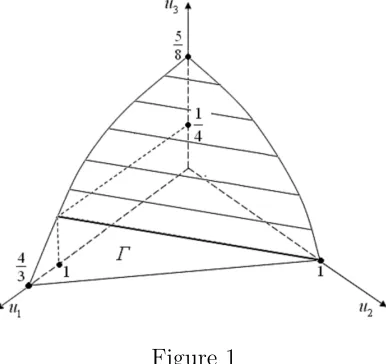
2 + 32u23 + 2u1u2 + 8u1u3 + 24u2u3 +u1 −4u2 − 20u3. The surface D00 given
by equation ϕ(u) = 0 is ruled (more precisely, it is part of a hyperbolic cylinder) and contains
segments of lines with a directing vectord = (4,−4,1) (see Fig. 1).
[image:13.612.209.402.217.399.2]Figure 1
The coordinates of x(a, u) from (25) are the following:
x1 =f(a)−u1, x2 =f(a)/2−(u1+ 2u2)/2, x3 =f(a)/4−(u1+ 2u2+ 4u3)/4.
By (23), (24), we getq(u) = 3u1+4u2+4u3,µ(a) = 9a/(1+a)−a,a∗ = 2,µ∗ = 4, ¯aF = 8. Hence the
set Γ, containing by Theorem 1 the setD0, is the nonnegative part of the plane 3u1+ 4u2+ 4u3 = 4.
By Corollary 2, u = (4/3,0,0)∈ D0. Indeed, ¯xu = (2/3,1/3,1/6)> 0. The equality p(u) = λ(a)
from (33) is equivalent to the following: u1 + 2u2 + 4u3 = 3a/(1 +a). By (34), the polyhedron
D(a) consists of nonnegative solutions of the following constraints system:
3u1+ 4u2+ 4u3 = 9a/(1 +a)−a, u1+ 2u2+ 4u3 ≤3a/(1 +a) (a∈[0,8]).
If in this system the inequality is replaced by an equality, then fora ∈[2,5] nonnegative solutions
of the resulting system give the set E(a). The set of vertices of this polyhedron consists of two
elements:
u1(a) = (3a/(1 +a)−a/2,0, a/8), u2(a) = (0,3a/(1 +a)−a/2, a/4−3a/4(1 +a)).
Hence, u1(a∗) = (1,0,1/4), u2(a∗) = (0,1,0). The line segment connecting these points (in Fig. 1
the thick line) is the boundary on the surface Dseparating the setsD0 (part of the plane) andD00,
and the segment itself belongs to the non-linear part of the surface — the set D00. The set E(a)
in complete agreement with Corollary 2 is the line segment joining the points u1(a) and u2(a):
E(a) = {u0+uα|α ∈[0,1]}(a∈[2,5]),
where u0 = (3a/(1 +a)−a/2, 0, a/8), uα = αa0(4,−4, 1), a0 = a/2−3a/4(1 +a) (in Fig. 1,
a series of parallel lines shows some of these sets).
Conclusion
In this article, we considered the properties of a feasible set for the problem of nondestructive use of renewable resources in the particular case of a nonlinear generalization of the Leslie model.
In the general case, for the problem (4) with concave map F, unfortunately, it has not yet been
possible to establish the existence of controls that preserve the structure of the ecosystem. But as we saw above (see Corollary 3), it turned out that in particular case of generalization of the nonlinear model Leslie, under concavity assumption of reproductivity function, such controls exist. In addition, we have established that such controls necessarily belong to a certain hyperplane. Moreover, the criterion is obtained that allows one to find such controls with certain properties.
For non-linear models with additive control, even for the model with a stationary withdrawal of individuals, one can not yet speak of the presence of a branched general theory, although properties of individual models have been well studied. Our general approach, which considers an ecosystem as an element of some general class of dynamic systems, also allows us to approach the problem of optimal exploitation of populations from fairly general positions. We hope that this study will show possible new directions in the development of the general theory of renewable resources exploitation.
Acknowledgements
This research was supported by Complex Program of Ural Branch of RAS, grant no. 18-1-1-17 and Russian Foundation for Basic Research, grant no.16-07-00266
References
[1] The State of World Fisheries and Aquaculture 2018. Meeting the sustainable development goals. Food and Agriculture, Organization of the United Nations. Rome (2018).
[2] V.S. Bezel’, V.F. Ishchenko, B.P. Popov, and S.S. Shvarts. Experience of mathematical simu-lation as applied to the ecological mechanisms in volved in the transformation of the genetic structure of populations, Doklady Akademii Nauk SSSR. 221, 964-966 (1975) (in Russian). [3] H. Caswell. Population Matrix Models: Construction, Analysis and Interpretation, 2nd edn.
Sunderland (Massachusetts, USA), Sinauer (2001).
[4] M. De Lara and L. Doyen. Sustainable Management of Natural Resources: Mathematical Models and Methods, Springer-Verlag, Berlin-Heidelberg (2008).
[5] W.G. Doubleday. Harvesting in matrix population model, Biometrics. 31 (1975), 189-200. [6] G.M. Dunkel. Maximum sustainable yields, SIAM J. Appl. Math. 19(2)(1970) 367-378. [7] W.M. Getz and R.G. Haight. Population Harvesting: Demographic Models of Fish, Forest,
and Animal Resources, Princeton University Press (1989).
[8] L.A. Goodman. The analysis of population growth when the birth and death rates depend upon several factors, Biometrics. 25 (1969) 659-681.
[9] D.R. Grey. Harvesting under density-dependent mortality and fecundity, J. Math. Biol. 26(2) (1988) 193-197.
[10] R. Law. A model for the dynamics of a plant population containing individuals classified by age and size, Ecology. 64 (1983) 224-230.
[11] L.P. Lefkovitch. The study of population growth in organisms grouped by stages, Biometrics. 21 (1965) 1-18.
[12] D. Logofet. Matrices and Graphs. Stability Problems in Mathematical Ecology, CRC Press (2018).
[13] D.O. Logofet and I.N. Belova. Nonnegative matrices as a tool to model population dynamics: classical models and contemporary expansions, J. Math. Sci. 155(6) (2008) 894-907 DOI: 10.1007/s10958-008-9249-2.
[14] Vl.D. Mazurov and A.I. Smirnov. On the reduction of the optimal non-destructive system exploitation problem to the mathematical programming problem, In: Evtushenko, Yu.G., Khachay, M.Yu., Khamisov, O.V., Kochetov, Yu.A., Malkova, V.U., Posypkin, M.A. (eds.): Proceedings of the OPTIMA-2017 Conference. 1987 (2017) 392-398.
[15] Vl.D. Mazurov and A.I. Smirnov. The conditions of irreducibility and primitivity monotone subhomogeneous maps, Trudy Instituta Matematiki i Mekhaniki UrO RAN. 22 (3)(2016) 169-177 DOI: 10.21538/0134-4889-2016-22-3-169-177.
[16] Vl.D. Mazurov and A.I. Smirnov. Properties of admissible set of an optimal non-destructive system exploitation problem in some general formalization, In: S. Belim, A. Kononov, Yu. Ko-valenko (eds.): Proceedings of the School-Seminar on Optimization Problems and their Ap-plications (2018) 359-371.
[17] H. Nikaido. Convex Structures and Economic Theory, Academic Press, NY (1968).
[18] W.J. Reed. Optimum age-specific harvesting in a nonlinear population model, Biometrics. 36(4) (1980) 579-593.
[19] A.I. Smirnov. Dynamics of the age-genetic composition of a biological population in a math-ematical model, Mathmath-ematical methods in the planning of industrial production. Trudy Insti-tuta Matematiki i Mekhaniki UNC AN USSR. 22 (1977) 91-98 (in Russian).
[20] A.I. Smirnov. On some nonlinear generalizations of Leslie model considering the effect of saturation, Bulletin of the Ural Institute of Economics, Management and Law. 4 (13) (2010) 98-101.
[21] O. Tahvonen. Age-structured optimization models in fisheries bioeconomics: a survey, In: R. Boucekkine, N. Hritonenko, Y. Yatsenko (eds). Optimal Control of Age structured Popu-lations in Economy, Demography, and the Environment. Routledge (2011) 140-173.
[22] M.B. Usher. A matrix approach to the management of renewable resources, with special reference to selection forests, J. Appl. Ecol. 3 (1966) 355-367.
[23] M.H. Williamson. Some extensions of the use of matrices in population theory, Bull. Math. Biophys. 21(1959) 13-17.