2019 International Conference on Information Technology, Electrical and Electronic Engineering (ITEEE 2019) ISBN: 978-1-60595-606-0
Group Consensus Analysis for Second Order Collective Model with
Spatial Coordinates Coupling
Fen NIE
1, Xiao-jun DUAN
2and Yi-cheng LIU
1,*1
Department of Mathematics, National University of Defense Technology, Changsha, 410073, P.R. China
2
Department of System of Systems, National University of Defense Technology, Changsha, 410073, P.R. China
*Corresponding author
Keywords: Multi-agent system (MAS), Rotation group consensus, Fixed topology, Directed graph.
Abstract. This paper focuses on the group consensus issue of multi-agent systems, where the agents in a network can reach more than one consistent values asymptotically. A rotation matrix is introduced to an existing consensus algorithm for double-integrator dynamics. Based on algebraic matrix theories, graph theories and the properties of Kronecker product, some necessary and sufficient criteria for the group consensus are derived. where we show that both the eigenvalue distribution of the Laplacian matrix and the Euler angle of the rotation matrix play an important role in achieving group consensus. Furthermore, we show that the agents will eventually keep moving on a linear pattern, cylindrical spiral pattern, and logarithmic spiral pattern when the damping gain is above a certain bound, the Euler angle is below, equal and above a critical value. simulated results are presented to demonstrate the theoretical results.
Introduction
In recent years, multi-agent systems have various applications in widely fields such as flocking or swarming in animal behaviors, energy networks and telecommunication networks, opinion systems and data mining. the coherent behavior of the agents caused the emerging phenomenon in terms of flocking and consensus, in which the agents reach final agreement on controlled variables of interest. There are many interesting research results on consensus problems for multi-agent systems[1]-[4]. However, Due to the changes of situations or cooperative tasks, the consensus values may be different for agents from different subnet-works, in [5], group consensus was introduced, where the states of all agents in the same sub-network reach the same consistent value while there is no agreement between any two sub-networks. group consensus problems for dynamic multi-agent systems were investigated by many researches[6]-[9], in [6], By introducing double-tree-form transformations, solve the first-order group consensus problems in networks of dynamic agents under switching topologies and when exist time-varying communication delays. in [7], By graph theories and matrix theories, solve the first-order group consensus problems of multi-agent systems with directed information exchange. in [8], By algebraic matrix theories, graph theories and the properties of Kronecker product, necessary and sufficient condition for the group consensus of multi-agent systems is established. in [9], By provided consensus protocols for double-integrator dynamic multi-agent systems solve the group consensus problems for networks with fixed communication topology. Inspired by the above analysis, this paper will investigate the group consensus of multi-agent model using a distributed protocol with Cartesian coordinate coupling matrix. The main contribution of this paper is to establish three flocking patterns with the rotation angle variation of coupling matrix.
This note is organized as follows. In Section 2, Some basic definitions and supporting results are presented. Section 3 contains the main results, and numerical results are presented in Section 4.
Notations. Throughout this paper, the following notations are used: the superscripts T stand for matrix transposition, respectively; [1,...,1]T
Preliminaries and Problem Formulation
Preliminaries
Let G =(V, E, A) be a weighted directed graph with a nonempty node set V = (v1,v2,...vnm), an edge
set VV, and a weighted adjacency matrix A. A=[aij](nm)(nm)is defined as aij 0ifeij
and else aij 0 . We assume aii 0 for alli . An edge eij (vj,vi)means that agent ican
receive information from agent j. A graph is called undirected ifaij aji. On the other hand, all
edges in a diagraph are ordered. A directed path is an ordered sequence ( , ),( , ),..., 3 2 2
1 i i i
i v v v
v where
) , (
1
k
k i
i v
v for all k. A diagraph is strongly connected if there is a directed path between any two distinct nodes. When the graph is undirected, strongly connected is called connected. The Laplacian matrixL[lij](nm)(nm)of graph G is defined as
m n
i j
j ij
ij ij
i j a
j i a l
,
1 , .
, ,
(1)
Problem Formulation
In this section, we consider the difference system
) ( ) (
) ( ) (
t u t v
t v t r
i i
i i
(2)
where ri(t):[xi(t),yi(t),zi(t)]TR3,vi(t):[vxi(t),vyi(t),vzi(t)]TR3,and ui(t) are the position, velocity and control input associated with the ith agent. Couple-group consensus requires that the first n agents reach one consistent value, whereas other m agents reach another consistent value. Denote l1 {1,2,...,n},l2{n1,n2,...,nm},ll1l2,Ek {eij |i, jlk}
). 2 , 1
(k Throughout the paper, we assume n1 and m1. Motivated by consensus protocols in [3],[9], the following consensus protocol is proposed:
2 1
2 1
2 1
) (
) (
)
( ) ( )
(
l
j ij j i j i
l
j ij j j
l
j ij j j
l
j ij j i j i
i
l i v v r
r C a v
r C a
l i v r C a v
v r
r C a t
u
(3)
where 0,aij 0,,if eijEk and aij 0,, if eijEk for all i,jlk,k 1,2;aijR,for all
2
1,j l
l
i or il2,jl1.
Definition 2.1 System (2) is said to reach couple-group consensus asymptotically if for any initial conditions, we have:
1
, ; 0 | |
lim , 0 | |
limt rirj t vivj i jl
2
, ; 0 | |
lim , 0 | |
limt rirj t vivj i jl
Before moving on, we make the following assumption as in ([5],[7])
Assumption 2.1 (a) 0, 1;
1a i l
m n
n
j ij
;(b) 1a 0, i l2.
n
j ij
In this paper, we assume that the information communication topology is time invariant and aij
is constant. The problem to be addressed in this paper is to establish conditions under which pattern can be achieved by applying proposed parameter.
Main Results
results of the paper. we aim to establish algebraic criteria for protocol (3) asymptotically solving the couple group consensus problem.
Let T m n n n T
n r r r r
r r r
r ( , ,..., ) , ( 1, 2,..., )
2 2 1 1
and ( 1, 2,..., ) ,
1 T
n
v v v
v v (vn 1,vn 2,...,vn m)T
2 , , ] ) ( , ) [( , ] ) ( , )
[(r1 T r2 T T v v1 T v2 T T
r then the system (2) can be written as
v r v r (4) With C L C L m n m n ) ( 3 ) ( 3 1 0 ) ( ) ( ]
[lij n m n m
L being defined as (1).
To proceed with the analysis, we first present a necessary lemma about L and restate its proof to derive two important vectors, which will be used in this paper.
Lemma 3.1 ([9]) Under Assumption 21, L has a zero eigenvalue whose geometric multiplicity is at least two.
. ] 1 , 0 [ , ] 0 , 1 [ 2 1 T T m T n T T m T n q
q (5)
1
q and q2 are two linearly independent right eigenvectors of L associated with zero
eigenvalues.
Definition 3.1 let i,i1,2,...,nm be the ith eigenvalue of L with associated right
eigenvectors i and an associated left eigenvector i and i 1 T i
, also let
0 )
arg(i fori 0, for all 0,arg( ) ( ,32)
2
i i , Without loss of generality, suppose that i
is labeled such that arg
1 arg
2 ...arg
nm
.where 12 0with associated righteigenvectors q1,q2 and an associated left eigenvector p1,p2 , where
T T T
p p
p1[ 11, 12] and
T T T
p p
p2 [ 21, 22] ,p1Tq1 1 and pT2q2 1. q1 and q2 are defined in (5).
Let ) 0 ( ) ( ), 0 ( ) ( ) 0 ( ) ( ), 0 ( ) ( ) | | ) Re( /( ) ( Im max 0 3 2 2 3 2 2 3 1 1 3 1 1 2 2 ,..., 3 v I p v r I p r v I p v r I p r T T T T i i i m n i
The eigenvalue and the eigenvectors of satisfy the following theorem.
Lemma 3.2 [2] Given a rotation matrix 3 3
CR , [ ,1 2, 3]
T
a a a a ( Without loss of generality,
assume a is a unit vector ) is the rotation axis, (0, 2 ) is the rotation angle. The eigenvalues of C is c1 1,
i
2 e
c ,c3 ei.When a a2, 3not all for zero, we choose the right eigenvectors of
C is 1a ,
2 2 T
2 [a2 a3, a a1 2 a3i, a a1 3 a2i]
, 3 2 , left eigenvectors
is 1 1, 2 2 22, 3 3 32, where i 1 is the imaginary unit , is the
conjugate of a complex number. we have lT l 1,l1, 2,3.
Lemma 3.3 [3] Consider the (n m ) ( n m)matrix L, the ith eigenvalue of L is given by i with associated right and left eigenvectors i and i, the eigenvalue of is given by
2
6( 1) (2i j 1) 3( 1)i j ( 3( 1)i j) 4 3( 1)i j / 2,
2
6( 1) 2i j 3( 1)i j ( 3( 1)i j) 4 3( 1)i j / 2,
with associated right eigenvectors :
6( 1) ( 2 1)
i j
i j i j
and 6( 1) 2
i j
i j i j
, with associated
left eigenvectors: 3( 1)
6( 1) (2 1)
i j i j
i j i j
and
3( 1)
6( 1) 2
i j i j
i j i j
, i1, 2,...,nm j, 1, 2,3, where
3i 2 i
, 3 1i iei
, 3i ie i
,whenL has an eigenvalue 0 of multiplicity two, LC has an eigenvalue 0 of multiplicity six, has an eigenvalue 0 of algebraic multiplicity twelve, geometric multiplicity six.
Theorem 3.1 If the matrixL has exactly zero eigenvalue of multiplicity two and all the other eigenvalues have positive real parts and 0 , Let the control algorithm for (2) be given by (3), then the following conclusion is established:
(i) Suppose that C I3, the couple-group consensus of multi-agent system (2) can be achieved,
furthermore, we have
lim[ ( ) (i k k )] 0, lim[ ( )i k ] 0, k, 1, 2.
t r t rtv t v t v i l k (6)
(ii) let ,
2
l i
and
3 ,
2
u i
be the two solution of
2 2
| i| cos( ) sin ( ) 0.
if
arg( ) ( ,3 /2)
| | min [ arg( )].
i
c u
i i
then the couple-group consensus of multi-agent system (2) can be achieved, then (6) is established.
(iii) Under the assumption of part 2, if | | c , and there exists a unique simple eigenvalue k
such that arg(k)[ ,3 / 2) and arg( ) .
u c
k k
then the group agents of l1 andl2 will
eventually move on circular orbits with the center given by r1tv1 and r2tv2 and the
period 2cot
ku , The radius of the orbit for the agents is given by2 ( ) [ (0), (0)]T T T T
k i p rc v
2 2 2
2 3 sin 2
a a . where k i( ) is the ith component of k and
2 3 1
3 1 2
1
6 3 2
k c
k k T
c
k k
p
where c
tan
ku /
i, The relative radius of the orbits is equal to the relative magnitudeof k i( ). The relative phase of the agents on their orbits is equal to the relative phase of k i( ).
(iv) Under the assumption of part 2, if there exists a unique simple eigenvalue k, such that
arg k [ ,3 / 2) , and ku arg(k)c and | | arg( ) [ ,3 /2),min [ arg( )]
i
c u
i i
i k
,then the
group agents of l1 andl2 will eventually move along logarithmic spiral curves with the center
given by r1tv1 and r2tv2, the growing rate Re(s), and the period
Im( s)
, The radius of the logarithmic spiral curve for the agents is given by
2 2 2
3 2 3 1 3 ( ) 2 3 2
[ci ( ),t ci( ),t c ti( )]T 2k i p rsT[ T(0),vT(0)]T a a sin
where ps p6k3,
2 2 4
2
s
with i
ke
.
3
n m n m
r r
v L L v
0 I
I
(7)
Note form lemma 33 that each eigenvalue i of the matrix L corresponds two eigenvalue of
give by 2 2 4
2 1 2
i i i
i
, with the associated right and left eigenvector given by, respectively
2 1
i
i i
and 2 1
i i
i i
and
2 2 4
2 2
i i i
i
, with the associated right and left eigenvector given
by, respectively
2
i
i i
and 2
i i
i i
, where i1, 2,...,nm, because the matrixL has
exactly zero eigenvalue of multiplicity two and all the other eigenvalues have positive real parts, we let 12 0 and Re
i 0 , i3, 4,...,nm .According to lemma 31, we can let1 q1, 2 q2,
and 1 p1,2 p2, According to lemma 33, has an eigenvalue 0 of algebraic
multiplicity four, geometric multiplicity two. without loss of generality. It thus follows that
1,2,3,4 0
with the associated the right eigenvector and the generalized right eigenvector given by,
respectively 1, [ ,0 ],1 3, [ ,0 ]2
T T
r r
w q w q and 2, [0 , ],1 4, [0 , 2]
T T
r r
w q w q , with the associated the
left eigenvector and the generalized left eigenvector given by, respectively
2, [0 , 1], 4, [0 , 2]
T T
l l
w p w p and 1, [ 1,0 ], 3, [ 2,0 ]
T T
l l
w p w p . Therefore, there exists a nonsingular
matrix 1
P P J , where Jis the Jordan canonical form. So we can obtain
1,
1
1, 4,
4,
0 1 0 0
0 0 0 0
,..., ,... 0 0 0 1
0 0 0 0
l
r r
l
w
PJP w w
w
J
0
0
0
0
0 0 0 0
Jis the diagonal matrix composed of Jordan blocks associated with the other eigenvalues of matrix except eigenvalues 0, by the sufficient and necessary conditions of [4] , when 0
, all the other nonzero eigenvalues of are in the open left half plane. so
11 12 11 12
1 21 22 21 22
11 12
21 22
lim 0
T T T T
T T T T
Jt
T T
t
T T
p p t p t p
p p t p t p Pe P
p p
p p
1 1 1 1
1 1 1 1
0 0 1 1
0 0 1 1
then
1 1
11 12 11 12
2 2
21 22 21 22 3
1 1
11 12
2 2
21 22
( ) (0)
( ) (0)
lim 0
( ) (0)
( ) (0)
T T T T
T T T T
T T
t
T T
p p t p t p
r t r
p p t p t p
r t r
I
p p
v t v
p p
v t v
1 1 1 1
1 1 1 1
0 0 1 1
0 0 1 1
so for i l kk, 1, 2, (6) is established. (ii) If 3 3
CR , then (4) can be written as
3(n m) 3(n m)
r r
v L C L C v
0 I
(8)
let 3 2 , 3 1 , 3 2 , 1, 2,...,
i i
i i i ie i ie i n m
Lemma 33 that each k corresponds to two eigenvalues of , given by
2 2
2k 1,2k k k 4 k / 2,k 1, 2,...,3(n m).
because 1 2 0 , it follows that
0, 1, 2,...,6,
i i
which in turn implies that i 0,i1, 2,...,12, Because all 2 2
4
k k
have
nonnegative real parts, it follows that all
2 2
2k k k 4 k / 2,k 1, 2,...,3(n m)
, have negative real
parts if c
. Give c
and arg( )
| | i i, 3, 4,...,( )
i i e i n m
, l
i
and iu are the critical values
for arg(i) [0, 2 ) such that
2 22k1 k k 4 k / 2
is on the imaginary axis. In particular, if
arg(i)il (respectively, iu), then
2 2
4 / 2 tan( l) /
k k k i i
(respectively, tan( u) / i
i
),
3, 4,...,
i nm ,if arg(i)
il, iu
(respectively, arg(i) [0, il),(iu, 2 ) ),then
2 2
4 / 2
k k k
has negative (respectively, positive) real parts. Because c
, the first
statement implies that all
2 2
4 / 2, 3, 4,...,
i i i i n m
,have negative real parts, which in turn
implies that arg(i)
il, iu
,i3, 4,...,nm, , if | | c , then arg(3i2),arg(3 1i) and3
arg(i)are all within
il, iu
, which implies that6i5,6i3 and 6 1i , i3, 4,...,nm,all havenegative real parts. Therefore, if | | c, then has exactly twelve zero eigenvalues and all other
eigenvalues have negative real parts k 0(k 1, 2,...,12), Re(k)0(k13,14,...,6(nm)) ,
meanwhile, by lemma 33, 1, [ 1 ,0 ], 3, [ 2 ,0 ]
T T
r j j r j j
w q w q and 2, [0 ,
T
r j
w q1
],
j
4, [0T , 2 ]
r j j
w q is the right eigenvector and the generalized right eigenvector of
associated with eigenvalue 0, 2, [0 , 1 ], 4, [0 , 2 ]
T T
l j j l j j
w p w p and w1,l [p1j,
0T j], 3, [ 2 ,0 ]
T
l j j
w p is the left eigenvector and the generalized left eigenvector of associated with eigenvalue 0.
Notice that
12 21 11 12
21 22 21 22
11 12
21 22
( )( ) ( )( ) ( )( ) ( )( )
( )( ) ( )( ) ( )( ) ( )( )
( )( ) ( )( )
( )( ) ( )( )
T T T T
j j j j j j j j
T T T T
j j j j j j j j
T T
j j j j
T T
j j j j
p p t p t p
p p t p t p
p p
p p
1 1 1 1
1 1 1 1
0 0 1 1
0 0 1 1
3
1
j
11 12 11 12
21 22 21 22
3
11 12
21 22
T T T T
T T T T
T T
T T
p p t p t p
p p t p t p
p p
p p
1 1 1 1
1 1 1 1
I
0 0 1 1
0 0 1 1
so as (ii) is established.
(iii) Still remember 3(n m) 3(n m)
L C L C
0 I
, Let us pretend that c
(when c
analysis methods are similar), if there is a unique simple eigenvaluek, make arg(k)[ ,3 / 2) ,
and c u arg( )
k k
, then 3 1 i | | ku
k ke k e
, by lemma 33, 6 3
tan /
u
k k i
, note
that the eigenvalue of are conjugated, so 6 3
tan /
u
k k i
, by lemma 33 choose the right
eigenvector associated with 6k3 is
2
6 3
6 3 2
k k
k k
q
. the left eigenvector is
3 3 1 6 3
3 1 2
1
6 3
6 3 2
k k
k k k
k k
p
and 6 3 6 3 1
T
k k
pair of pure imaginary eigenvalues of , all the other nonzero eigenvalues of are in the open left half plane.
( ) (0)
( ) (0)
t
r t r
e
v t v
that is
1 1
11 12 11 12
2 2
21 22 21 22 3
1 1
11 12
2 2
21 22
( ) (0)
( ) (0)
lim ( ) 0.
( ) (0)
( ) (0)
T T T T
T T T T
T T
t
T T
p p t p t p
r t r
p p t p t p
r t r
I c t
p p
v t v
p p
v t v
1 1 1 1
1 1 1 1
0 0 1 1
0 0 1 1
where
(tan )/ (tan )/
6 3 6 3 6 3 6 3
(0)
( ) [ ] .
(0)
u u
kti T kti T
k k k k
r
c t e q p e q p
v
let c tk( ) be the kth component of c t k( ), 1, 2,...,6(nm).
3( 1) cos[ (tan / ) arg ( ) 6 3[ (0), (0)] arg( 2( ))]
u T T T T
i j k k i k j
c r t p r v
where
2( ) ( ) 6 3
2 T [ T(0), T(0)]T
j k i k
r p r v .
2( )j
is the j component of2,k i( ) is the i component of k,i1, 2,...,nm, j1, 2,3,The radius of the
orbit for agent i is given by
2 2 2
3 2 3 1 3 ( ) 6 3 2 3 2
[ ( ), ( ), ( )]T 2 T [ T(0), T(0)]T sin
i i i k i k
c t c t c t p r v a a
so, the group agents of ofl1 andl2 will eventually move on circular orbits with the center given
byr1tv1 and r2tv2 and the period 2 cot
u k
, The radius of the orbit for the agents is given by
2 2 2
( ) 6 3 2 3 2
2 T [ T(0), T(0)]T sin
k i p k r v a a
(iv) For the fourth statement, If there exists a unique simple eigenvalue k , such that
arg k [ ,3 / 2) , and ku arg
k c , and | | arg min[ ,3 /2), arg
i
c u
i i
i k
then
6k 3
3 1
2 2
3k 1 k 4 3k 1 / 2
with positive real parts, similar to the analysis of the third
statement, has an eigenvalue 0 of algebraic multiplicity twelve, geometric multiplicity six, has two eigenvalue with positive real parts, and all other eigenvalues have negative real parts. then
1 1
11 12 11 12
2 2
21 22 21 22 3
1 1
11 12
2 2
21 22
( ) (0)
( ) (0)
lim ( ) 0.
( ) (0)
( ) (0)
T T T T
T T T T
T T
t
T T
p p t p t p
r t r
p p t p t p
r t r
c t
p p
v t v
p p
v t v
1 1 1 1
1 1 1 1
I
0 0 1 1
0 0 1 1
where
6 3 6 3
6 3 6 3 6 3 6 3
(0)
( ) [ ] .
(0)
k t T k t T
k k k k
r c t e q p e q p
v
letc tk( )be the kth component of c t( ), k 1, 2,...,6(nm)
Re( )
3( 1) cos[Im( ) arg ( ) 6 3[ (0), (0)] arg( 2( ))]
st T T T T
i j s k i k j
c re t p r v
where
4
/ 2, i| |s ke
. then the group agents of l1 andl2 will eventually
move along logarithmic spiral curves with the center given by r1tv1 and r2tv2, the
growing rate Re(s), and the period 2 Im( s)
Re( ) 2 2 2
3 2 3 1 3 ( ) 6 3 2 3 2
[ ( ), ( ), ( )]T 2 T [ T(0), T(0)]T s t sin
i i i k i k
c t c t c t p r v e a a
Numerical Simulation
In this section, the main conclusions of the article are verified by numerical simulation. In the numerical simulation, the number of agents is assumedn7.
3 3 0 1 0 0 1
2 3 1 1 0 0 1
1 0 1 0 0 0 0
1 1 0 2 0 0 2
0 0 0 1 1 0 0
0 0 0 0 1 1 0
1 1 0 2 0 1 3
L
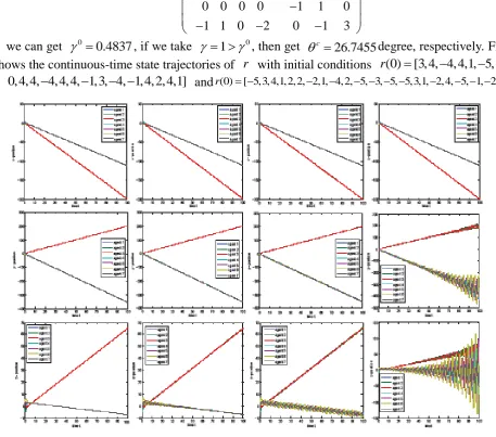
we can get 0 0.4837, if we take 1 0, then get c 26.7455degree, respectively. Fig.1 shows the continuous-time state trajectories of r with initial conditions (0)r [3, 4, 4, 4,1, 5, 3,
0, 4, 4, 4, 4, 4, 1,3, 4, 1, 4, 2, 4,1] andr(0) [ 5,3, 4,1, 2, 2, 2,1, 4, 2, 5, 3, 5, 5,3,1, 2, 4, 5, 1, 2] .
Figure 1: x y z, , direction trajectory of 7 agents, The 3 subgraph of the first column
with 0degree, the second column with
90
c
=0.4319(24.7455 degree), the third column with
c
= 0.4668(26.7455 degree), the fourth column with
90
c
=0.5017(28.7455 degree).
Acknowledgements
[image:8.595.63.521.253.656.2]References
[1] Olfatisaber R, Murray R M. Consensus problems in networks of agents with switching topology and time-delays[J]. IEEE Transactions on Automatic Control, 49(9):1520-1533, (2004).
[2] REN W, Cao Y. Distributed Coordination of Multi-Agent Networks: Emergent Problems, Models, and Issues[J]. Communications Control Engineering, (2010). 11
[3] Yi-cheng LIU, Xiang LI, Fen NIE. Analysis for second-order collective model with spatial coordinates coupling[J].Journal of National University of Defense Technology, 39(6): 118-125 (2017).
[4] Yu, W., Chen, G., Cao, M. Some necessary and sufficient conditions for second-order consensus in multi-agent dynamical systems. Automatica, 46(6), 1089-1095. (2010).
[5] Yu J, Wang L. Group consensus of multi-agent systems with undirected communication graphs[C] Asian Control Conference. Ascc 2009. IEEE:105-110.(2009).
[6] Yu JY, Wang L. Group consensus in multi-agent systems with switching topologies and coummunication delays. Systems Control Letters; 59(6): 340`C348 (2010).
[7] Yu JY, Wang L. Group consensus of multi-agent systems with directed information ex-change[J]. International Journal of Systems Science, 43(2):334-348, (2012).
[8] Xie D, Liu Q, Lv L, et al. Necessary and sufficient condition for the group consensus of multi-agent systems[J]. Applied Mathematics Computation, 243: 870-878, (2014).