Improving the Performance of a Power Hardware In the Loop System by a New Interface Algorithm

2018 International Conference on Applied Mechanics, Mathematics, Modeling and Simulation (AMMMS 2018) ISBN: 978-1-60595-589-6

Improving the Performance of a Power Hardware-In-the-Loop

System by a New Interface Algorithm

Chen-xu YIN

*, Bin YE

, Liu-zhu ZHU

, Jing MA

, Xu-li WANG

,

Lei DAI

and Lu-yao MA

1_{State Grid Anhui Economic Research Institute, Hefei China 230022}

2_{State Grid Anhui Electric Power CO. LTD. Hefei China 230061}

3_{State Grid Anhui Training Center, Hefei China 230000}

Keyword: Power hardware-in-the-loop, Interface algorithm, Virtual impedance method,

Performance.

Abstract. Power Hardware-In-the-Loop (PHIL) is an efficient way to analysis and test electrical equipment which is introduced into power system. To improve the performance of a PHIL system, the feasibility of several interface algorithms for PHIL system are analyzed. And a new interface algorithm, which is based on the virtual impedance method (VIM), is proposed. Therefore, the proposed interface algorithm is compared and assessed with the current interface algorithms. Through the comparing and testing, the proposed interface algorithm is verified that it obtains a better overall performance than another.

Introduction

With a rapid development of smart grid technology, amount of the power electronic equipment connecting to power grid, such as distributed generation, micro-grid, electric vehicles and other new technologies, many new devices will be introduced into the future power system. How to test and analyze the new devices poses new challenges to the traditional simulation methods. Power Hardware-In-the-Loop (PHIL) simulation [1], which combines the electrical equipment under test (EUT) and digital simulation (DS), is capable of testing the actual power devices. As a new trend of a power system simulation technology, a PHIL simulation is of great research value and has a wide application prospect. PHIL simulations allow the prototype of a novel apparatus to be investigated in a virtual system under a wide range of realistic conditions repeatedly, safely, and economically.

The interface algorithm is an efficient way to improve the performance of a PHIL system. A HVDC simulation model has been established on RTDS according to [2], and through the analyze and testing, the transmission line mode (TLM)l interface algorithm has been recommend for PHIL system; An ideal transformer method (ITM) interface algorithm model is analyzed in [3]. The feasibility of a time-varying first order approximation method (TFA) has been analyzed[4]. Several interface algorithm models are compared on literature[5]. A damping impedance method (DIM) model has relatively good stability and accuracy. However, through the study of the current literatures, most of the current interface algorithms are poor in practicability or performance of the PHIL simulations[6].

To improve the performance of a PHIL system, the applicability of the different interface algorithms and their influences on the performance of a PHIL system are analyzed. And a new interface algorithm, which is based on a virtual impedance method, is proposed. Therefore, the proposed interface algorithm is compared and assessed with the current interface algorithms. Through the analysis and PHIL simulations, the proposed algorithm is confirmed that it achieves a better overall performance than another.

Modeling of a PHIL System

model of the electrical equipment under the test (EUT) and the a power interface model, and a power interface (PI) part contains the disturbance factors of the PHIL system.

Vs(s) I2' (s) V₁'(s)

I2(s)

DS EUT

V1(s)

Z2(s)

Z1(s)

V2(s)

PI

Rl

GDA(s) Gp(s) GAD(s)

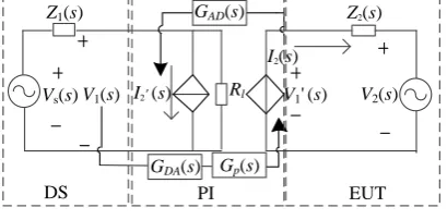
Figure 1. A PHIL system.

To analysis the modeling method, taking the first order linear circuit model as an example, the block diagram of the equivalent PHIL system, which is based on the voltage type ideal transformer method(ITM) model, is set up as shown in Fig.1. The voltage source V1 (s) is series with an

impedance Z1(s) on DS. It can be equivalent to the voltage source V2(s) is series with a load

impedance Z2(s) on EUT. The equivalent model of PI is controlled by the voltage source V1'(s), and

the output current of the measured device is used as feedback signal to control the controlled current source I2' (s), and Rl is its infinite internal resistance. The digital signal and the analog signal are

interacted, so the DA link is equivalent to GDA(s). Meanwhile, the equivalent transfer function is

Gp(s), and thus the PHIL model system can be obtained. The open loop transfer function GOL(s) of

the system is described:

1

2

( ) ( ) ( ) ( )

( )

OL DA p

Z s

G s G s G s

Z s

 (1)

The block diagram of a transfer function for PHIL system is shown in Fig. 2.

+

+ _

Vs(s) _{G 1/Z2(s)} V2(s)

DA(s) Gp(s) I2(s) I2'(s)

V1'(s)

1/Z2(s)

GDA(s) _

Z1(s)

Vf(s)

DS PI EUT

Figure 2. A transfer function of a PHIL system.

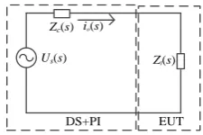
An impedance model of a PHIL system can be study by analyzing the impedance characteristics of the system.

+

— Uref(s)

Gc(s) KPWM 1

o

L s —

+ 1

o

C s

Uo(s) io(s)

ic(s)

kc —

+ _G

d(s)

+

Us(s)

GDA(s) —

Zs(s) GDA(s) if(s)

DS PI

Figure 3. A transfer function of a PHIL system.

The PI is based on the continuous small signal linear model under the control block diagram as shown in Fig.3. Gc(s) is a power interface controller, GDA(s) is an equivalent conversion model, KC

is an active damping capacitance current feedback coefficient, KPWM is the equivalent gain of the

inverter, and Gd(s) is a transfer function of the time delay equivalent model of a power interface.

Us(s)

Gz1(s) Gz2(s)

Uo(s) Io(s)

Figure 4. An equivalent control block diagram.

According to Mason's method, the equivalent control block diagram of the PHIL system is obtained in Fig.4

( ) ( ) ( )

( ) KPWM G s Gd DAs G sc

2 2

( ) ( ) ( ) ( ) ( )

( ) ( ) ( )

o PWM s c DA d

z

o o o PWM c d PWM d c

L s K Z s G s G s G s

G s

L C s C s K K G s K G s G s

  



      ₍₃₎

The output voltage Us(s) can be equivalent as follow:

'

1 2 2

( ) ( ) ( ) ( ) ( ) ( ) ( ) ( ) ( )

o z z s z o s o o

U s G s G s U s G s I s U s Z s I s ₍₄₎

It is obtained by formula (3.4) that an equivalent PHIL system is divided into two parts, one part is the output voltage source U's(s). Its output dynamic performance is mainly determined by the

controller of a PI; The other part is the output of a PHIL system. The impedance Zo(s), which

includes the delay part, the power interface controller and the output filter, is influenced the overall impedance characteristics of a PHIL system. Therefore, the equivalent circuit of a PHIL system is obtained, as shown in Fig.5.

Us(s)

Zo(s) Io(s)

+

+

Uo(s)

´

Us(s)

io(s)

Zc(s)

Zl(s)

EUT DS+PI

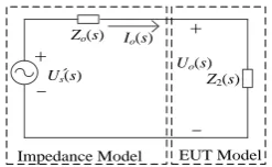
Figure 5. An equivalent circuit. Figure 6. An equivalent impedance PHIL model.

The Us(s) is the equivalent voltage source. When the voltage base wave instruction is given to 0,

and the output current is given a certain frequency current on DS part. Therefore, the output voltage and output current ratio is the output impedance Zo(s) of a PHIL system.

Stability Analysis

According to the impedance PHIL model shown in Fig.4, the equivalent circuit is shown in Fig.6. The DS system and the PI are equivalent to an impedance Zc(s).

According to Kirchhoff's method, the output current IO(s) and voltage source Us(s) can be

obtained as follow:

( ) ( )

( ) ( )

s o

l c

U s i s

Z s Z s



 ₍₅₎

The further equivalent is shown as follow：

( ) 1

( )

( ) 1 ( ) / ( )

s o

l c l

U s i s

Z s Z s Z s

 

 ₍₆₎

The voltage source US(s) can be stable operated under open circuit condition, and a load Zl(s) has

no right half plane pole, so the stability of PHIL system depends on:

1 ( )

1 c( ) / l( )

H s

Z s Z s



 ₍₇₎

The transfer function H(s) is represented as a closed loop system, as shown in Figure 7.

+

Zc(s)/Zl(s)

Figure 7. An equivalent impedance PHIL mode.

Therefore, the stability of a PHIL system is determined by the closed loop transfer function H(s). A stability criterion of the classical control theory is introduced to evaluate the stability of the system. The criterion method can also be applied to nonlinear equipment simulations.

A New Interface Algorithm

impedance model, which makes the equivalent output impedance of the system close to the impedance of an original circuit, to improve the performance of a PHIL system.

Us(s)

Zo(s) Io(s)

+

+

Uo(s) ´

Impedance Model EUT Model

Z2(s)

Figure 8. An equivalent impedance PHIL model.

An impedance model of a PHIL system is shown in Figure8 and the expression is obtained according to the circuit topology.

'

( ) ( ) ( ) ( )

o s o o

U s U s Z s I s _(8).

And the Us’(s)and Zo(s)can be obtained based on the former analysis.

'

2

1 2

( ) ( ) ( ) ( ) ( )

( ) ( ) ( )

( ) ( ) ( ) ( ) ( )

( ) ( ) ( )

PWM d DA c s

s

o o o PWM c d PWM d c

o PWM c DA d

o

o o o PWM c d PWM d c

K G s G s G s U s U s

L C s C s K k G s K G s G s

L s K Z s G s G s G s Z s

L C s C s K k G s K G s G s

 _ 

 _{     }

 

  

 _

      

 _(9). '

Gi(s) 1/Z2(s)

Uo(s)

Z1(s)

Us(s)+

'

Gi(s) 1/Z2(s)

Uo(s)

Z1(s)

Us(s)+

Zo(s)

(a)S-domain transfer function (b) S-domain transfer function

Figure 9. An equivalent transfer function.

A PHIL system structure has been shown in Figure9, Gi(s) is the equivalent model of the power

interface, the output impedance Zo(s) of a PHIL system can be represented as:

1

( ) ( ) ( )

o i

Z s Z s G s ₍₁₀₎

The output impedance model contains an interface part, delays and errors. To eliminate the amount of disturbance in the output impedance, a VIM interface algorithm is introduced.

Us(s)

Zo(s) Io(s)

+

+

Uo(s)

´

´

Impedance Model EUT Model

Zc(s)

Z2(s)

Figure 10. An equivalent circuit.

According to the circuit theorem, the output impedance Zo(s)can be corrected and compensated

by a series impedance. As shown in Figure10, the virtual impedance Zc(s) is introduced in series

with Zo(s), and the compensated impedance Zeq(s) can be obtained:

1

( ) ( ) ( ) ( )

eq c o

Z s Z s Z s Z s

(11) Therefore, the series compensation impedance can be expressed as:

1 1

( ) ( ) ( ) ( ) ( )

c o o

Z s Z s Z s Z s T s ₍₁₂₎

The To(s) simplification is equivalent as follow:

2

( ) ( ) ( ) 1

( ) ( ) ( )

PWM c d

o

o o o PWM c d PWM d c

K G s G s

T s

L C s C s K k G s K G s G s

  

The transfer function of a PHIL system with series impedance can be obtained based on the impedance model shown in Figure10, which is shown in Figure 11(a) and Figure 11 (b).

1/Z2(s)

Uo(s)

Z1(s)

+

Zc(s)

+ Us´(s)

+ GPI(s)

Zo(s)

VIM Model

1/Z2(s) Z1(s)

Zc(s) 1/Z1(s)

Us´(s) Uo(s)

+ +

DS

Gs(s)

+

1/GPI(s)

GPI(s)

(a) S-domain transfer function (b) S-domain transfer function

Figure 11. The PHIL system structure.

The PHIL structure with the virtual impedance ZC(s) is added. Therefore, the equivalent

expression of the equivalent transfer function compensation is expressed:

2

2

( ) ( ) ( ) ( )

( )

o o o PWM c d PWM d c

VIM

o o o PWM c d

L C s C s K k G s K G s G s

G s

L C s C s K k G s

     



    ₍₁₄₎

DS

Ri

Interface Algorithm

Grid

i2´

GVIM(s)

i1

Figure 12. The PHIL system on VIM model.

As shown in Figure12, the impedance model GVIM(s) is set on DS side, the current I2 is fed to the

DS by the measured device, and the current I1 is a controlled current source of DS, which Ri is

parallel to the infinite impedance of the controlled current source, without changing the circuit structure, increasing the impedance value or other equipment, and comparing the other power interface algorithm, the VIM model has strong flexibility and it is simple established on the real-time digital simulation software.

Experimental Verification

A PHIL Platform

EUT

R2 L2 Us

R1

DS

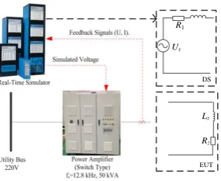
Figure 13. The PHIL system platform.

To verify the efficacy of a VIM interface algorithm, a PHIL platform is established, which is shown on Figure13. The voltage source Usis 220V, R1 and L1 are impedance and resistance, which

are series with the voltage source Us on the DS side, two parts are split into the DS and the EUT,

based on the TLM model; The inductor L1 is equivalent to the line impedance, which is split into

Stability Analyze

The TFA method is calculated based on the prediction data, thus this paper does not analyze and test the TFA method. For another interface algorithms, such as TLM, DIM, PCD and ITM, it has relatively good practicability and feasibility. Therefore, several interface algorithms and the VIM is used to analyze and compare the performance of a PHIL system.

Taking the first order circuit, which is shown in Figure15, as an example, the power supply voltage USis 220V. The power interface parameters are shown in Table. 1

Table 1. The parameters of a PHIL system.

Filter Parameters Controller DC voltage

Lo(mH) Co(μF) kp kf ks kc Udc(V)

0.2 60 5 0.95 1.5 2 500

Two different circuit impedance parameters are shown in Table. II

Table 2. The parameters of the impedance.

Parameter R1(Ω) L1(mH) R2(Ω) L2(mH)

Group 1 4 40 4 80

Group 2 4 80 4 40

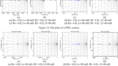
Figure 14 (a) shows the poles of a PHIL system based on the ITM method only exist in a group 1, and the system can be stable. Figure 14 (b) shows there is a positive real part of the system, and it is unstable. Because the impedance ratio, between the DS side and HUT, is greater than 1. As shown in Figure15 and Figure16, the poles of the simulation model based on the PCD, TLM DIM and VIM only have the negative real part, and the system can be stable.

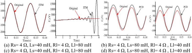
Figure17, Figure18 and Figure19 show that several interface algorithms can be stable under the current simulation parameters and circuit structures, the error voltage waveform between a PHIL system and an original system can be obtained. The better simulation accuracy of the PHIL system, based on the ITM, DIM and VIM, have been obtained. Therefore, the VIM have relatively stability, accuracy and feasibility overall the performance.

Pole-Zero Map Real Axis Im a g in a ry A x is

-100 -80 -60 -40 -20 0

-1 -0.5 0 0.5 1

-300 -200 -100 0 100 200 300

-1 -0.5 0 0.5

1 Pole-Zero Map

Real Axis Im a g in a ry A x is

-100 -50 0

-1 -0.5 0 0.5 1 Real Axis Im ag in ar y A x is Pole-Zero Map

-100 -50 0

-1 -0.5 0 0.5 1 Real Axis Im ag in ar y A x is Pole-Zero Map

(a) (b) (c) (d) (a) Rs= 4 Ω, Ls=40 mH, Rl= 4 Ω, Ll=80 mH (b) Rs= 4 Ω, Ls=80 mH, Rl= 4 Ω , Ll=40 mH (c) Rs= 4 Ω, Ls=40 mH, Rl= 4 Ω, Ll=80 mH (d) Rs= 4 Ω, Ls=80 mH, Rl= 4 Ω , Ll=40 mH

Figure 14. The poles of a PHIL system.

-3000 -2000 -1000 0

-1 -0.5 0 0.5 1 Real Axis Im ag in ar y A x is Pole-Zero Map

-10000 -5000 0

-1 -0.5 0 0.5 1 Real Axis Im ag in ar y A x is Pole-Zero Map

-100 -50 0

-1 -0.5 0 0.5 1 Real Axis Im ag in ar y A x is Pole-Zero Map

-100 -50 0

-1 -0.5 0 0.5 1 Real Axis Im ag in ar y A x is Pole-Zero Map

(a) (b) (c) (d) (a) Rs= 4 Ω, Ls=40 mH, Rl= 4 Ω, Ll=80 mH (b) Rs= 4 Ω, Ls=80 mH, Rl= 4 Ω , Ll=40 mH (c) Rs= 4 Ω, Ls=40 mH, Rl= 4 Ω, Ll=80 mH (d) Rs= 4 Ω, Ls=80 mH, Rl= 4 Ω , Ll=40 mH

-100 -80 -60 -40 -20 0 -1

-0.5 0 0.5

1 Pole-Zero Map

Im ag in ar y A x is Real Axis

-100 -80 -60 -40 -20 0 -1 -0.5 0 0.5 1 Real Axis Im ag in ar y A x is Pole-Zero Map

(a) (b)

(a) Rs= 4 Ω, Ls=40 mH, Rl= 4 Ω, Ll=80 mH (b) Rs= 4 Ω, Ls=80 mH, Rl= 4 Ω , Ll=40 mH

Figure 16. The poles of a PHIL system.

PHIL Simulations

0.1 0.11 0.12 0.13 0.14

-200 -100 0 100

200 _{Original ITM}

Time(s) Uo

(V

)

0 1 2 3 4 5 6 -1000 -500 0 500 1000 1500 T(ms) U o (V ) Original ITM

0.14 0.15 0.16 0.17 0.18 -300 -200 -100 0 100 200 300 Original PCD Uo (V )

time(s) 0.12 0.13 0.14 0.15 0.16 -100

-50 0 50 100

150 Original PCD

Uo

(V

)

Time(s)

(a) Rs= 4 Ω, Ls=40 mH, Rl= 4 Ω, Ll=80 mH (b) Rs= 4 Ω, Ls=80 mH, Rl= 4 Ω , Ll=40 mH (c) Rs= 4 Ω, Ls=40 mH, Rl= 4 Ω, Ll=80 mH (d) Rs= 4 Ω, Ls=80 mH, Rl= 4 Ω , Ll=40 mH

Figure 17. The performance of the ITM and PCD model.

0.1 0.11 0.12 0.13 0.14

-200 -100 0 100 200 Uo (V ) TLM Original

Time(s) 0.1 0.11 0.12 0.13 0.14

-150 -100 -50 0 50 100 150 TLM Original U o (V ) Time(s)

0.12 0.13 0.14 0.15 0.16

-200 -100 0 100

200 Original _DIM

U

o

(V

)

Time(s) 0.12 0.13 0.14 0.15 0.16

-150 -100 -50 0 50 100 150 DIM Original Uo (V ) Time(s)

(a) Rs= 4 Ω, Ls=40 mH, Rl= 4 Ω, Ll=80 mH (b) Rs= 4 Ω, Ls=80 mH, Rl= 4 Ω , Ll=40 mH (c) Rs= 4 Ω, Ls=40 mH, Rl= 4 Ω, Ll=80 mH (d) Rs= 4 Ω, Ls=80 mH, Rl= 4 Ω , Ll=40 mH

Figure 18. The performance of the TLM and DIM model.

0.12 0.13 0.14 0.15 0.16 -200

-100 0 100

200 Original _VIM

Uo

(V

)

Time(s)

0.12 0.13 0.14 0.15 0.16 -150 -100 -50 0 50 100 150 VIM Original Uo (V ) Time(s)

(a) Rs= 4 Ω, Ls=40 mH, Rl= 4 Ω, Ll=80 mH (b) Rs= 4 Ω, Ls=80 mH, Rl= 4 Ω , Ll=40 mH

Figure 19. The performance of a VIM model.

Conclusion

References

[1] Wang, J., Song, Y., Li, W., Guo, J., and Monti, A.: ‘Development of a Universal Platform for Hardware In-the-Loop Testing of Microgrids’, IEEE Transactions on Industrial Informatics, 2014, 4, (10), pp. 2154-2165.

[2] Steurer, M., Edrington, C., Sloderbeck, M., Ren, W., and Langston, J.: ‘A megawatt-scale power hardware-in-the-loop simulation setup for motor drives’, IEEE Transactions on Industrial Electronics, 2010, 4, (57), pp. 1254-1260.

[3] Hong M, Chien-ru L, Miura Y, et al. Accuracy evaluation of power hardware-in-the-loop simulation of a boost chopper[C]. Power Electronics Conference (IPEC), 2010 International. IEEE, 2010: 2424-2429.

[4] Ren W, Steurer M, Baldwin T L. Improve the stability and the accuracy of power hardware-in-the-loop simulation by selecting appropriate interface algorithms[J]. IEEE Transactions on Industry Applications, 2008, 44(4): 1286-1294.

[5] Viehweider A, Lehfuss F, Lauss G. Interface and stability issues for SISO and MIMO power hardware in the loop simulation of distribution networks with photovoltaic generation[J]. International Journal of Renewable Energy Research (IJRER), 2012, 2(4): 631-639.

[6] Hui, L., Steurer, M., Shi, K. L., Woodruff, S., and Da, Z.: ‘Development of a unified design,