Method for Medium speed Maglev Train Timetabling with Consideration of Passenger Demands

2018 3rd International Conference on Computational Modeling, Simulation and Applied Mathematics (CMSAM 2018) ISBN: 978-1-60595-035-8

Method for Medium-speed Maglev Train Timetabling with Consideration

of Passenger Demands

Shu-qin HUO

1

, Ling-yun MENG

1

, Qing-ying LAI

2

, Jun LIU

1

,

Lu LIU

1

and Ya-zhi XU

3

1_{School of Traffic and Transportation, Beijing Jiaotong University, Beijing, 100044, China}

2 _{State Key Laboratory of Rail Traffic Control and Safety, Beijing Jiaotong University,}

Beijing 100044, China

3_{CRRC Tangshan Co., Ltd –R & D center, Tangshan 064000, China}

Keywords: Medium-speed maglev train, Passenger demands, Train timetable, Lagrange relaxation.

Abstract. Medium-speed maglev train serves for suburban passenger flow, and it’s important to research on medium-speed maglev train timetabling with consideration of passenger demands, but there is still no research in this area. Combing the passenger flow scenes for medium-speed maglev traffic and the occupancy characteristics of operation resources, a study on the timetabling of medium-speed maglev train considering passenger demands is conducted in this paper. The timetabling problem is formulated as a 0-1 integer programming model based on cumulative flow variables with the objective of minimizing the total travel time for passengers, and the Lagrange relaxation algorithm is used to solve the model. Finally, the model and algorithm are analyzed and verified by a numerical experiment.

Introduction

With the acceleration of China's urbanization process, the medium-speed maglev (MSM) with a speed of 200 kilometers per hour, as a new type of rail transit with green, low cost and high service quality, will play an important role in the demand for commuter passenger flow in the suburbs.

At present, research on train timetabling of railways and urban rail transit is abundant[1,2], which aims to solve the problem from maximizing revenue of railways[3], to consider passengers’ satisfaction in many aspects[4,5]. In comparison, the maglev system has the following characteristics: (1) Only one train is allowed to operate in the same power supply zone (PSZ)[6] at the same time; (2) Medium-speed and high-speed maglev need to set up auxiliary stopping areas (ASA)[6] in the PSZ to ensure that the maglev train has enough energy to suspend under accidental conditions; (3) There is no need to set up skylights for the maglev system to maintain maglev line or train in the early design stage; (4) Because of the suspension, the train has strict limitations on the carrying capacity. Therefore, the method of traditional train timetabling is not suitable for the maglev train timetabling. In addition, the conferences[7,8] proposed the method for high-speed maglev train timetabling without considering the influence of ASA.

In this paper, we first describe the condition of medium-speed maglev traffic, and model the operation process of MSM train as occupancy of operation resources (OR). Then, we strictly limit passenger's expecting departure and arrival time spans, a model of MSM train timetabling is proposed in this paper. Finally, the model and algorithm is analyzed and verified by a numerical experiment.

A Model for Medium-Speed Maglev Train Timetabling

A. Infrastructure Description and Modeling of Operation Resources Occupancy

path is regarded as cells set, as shown in Figure 1, and all trains in down direction use the routes in Figure 2.

The occupancy characteristics of PSZ is described as "R i j

 

, ", and the train headway time is

regarded as the time of occupyingR i j

 

, . We use the "blocking time model" to indicate the time of [image:2.595.89.509.183.309.2]

occupyingR i j

 

, , as shown in Figure 3. Comparing to the railway system, the time for the train to run from the ASA to the target PSZ is added into the MSM system’s blocking time, as "Approach time 2" in Figure 3.

Figure 1. A simple Maglev line

1 2 3 4

5 7

6 8 9

12 13 14

15

16 17 Down

10 11 Siding track

Route 1 Route 2 Route 3 Route 4

1 2 3 4

5 7

6 8 9

12 13 14

15

16 17

34 32

31 30 29

28

27 25 24

23 22 21

20

19 18 Down

10 11

26 33

Turnout conversion point Siding track

ASA

Setup time Reaction time Approach time 1

Running time Clearing time Release time

max

v v

s

t

Common braking curve

Cue point

H

L

Setup time

C

T Reaction time TD

A

T Approach time 1 Approach time 2TH

O

T Running time Clearing time

U

T

I

T

Release time Blocking time TB

Power Supply Zone (PSZ) Auxiliary Stopping Area (ASA)

ASA

Figure 2. Line information and stopping scheme. Figure 3. Occupancy time schematic of OR.

The actual occupancy time of R i j

 

, is earlier than the time when the train arrives. The time for

trains to release R i j

 

, is later than the time when the train leaves. Therefore, parameters h_{f i j, ,}

and ' , , f i j

h are introduced to describe the actual occupancy of R i j

 

, ,

where '

, , , , ,

f i j I D A H f i j C U

h T T T T h T T . Among them, h_{f i j, ,} indicates the time interval between occupying R i j

 

, and entering R i j

 

, , '

, , f i j

h indicates the time interval between releasing

 

,

R i j and departing fromR i j

 

, . [image:2.595.85.517.471.706.2]

B. Notation

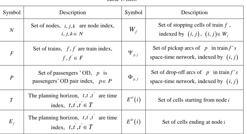
Table 1. Sets.

Symbol Description Symbol Description

N Set of nodes, i j k, , are node index,

, ,

i j kN Wf

Set of stopping cells of train f , indexed by  i j, ,  i j, W_f

F Set of trains,

'

,

f f are train index,

'

,

f f F p f,

Set of pickup arcs of p in train f’ s space-time network, indexed by  i j,

P _{passengers’ OD pair index,} Set of passengers ’ OD, p is

pP p f,

Set of drop-off arcs of p in train f’ s space-time network, indexed by  i j,

T The planning horizon, ' ''

, ,

t t t are time

index, t t t, ,' ''T  

O

E i Set of cells starting from nodei

f

E The planning horizon, ' ''

, ,

t t t are time

index, t t t, ,' ''T  

D

Table 2. Input parameters.

Symbol Description Symbol Description

f

 Maximum passenger volume that

train f can load Ap Arriving time of passenger group p

e f

 , l_f The earliest and latest departing _{time of train}

f in origin station p Volume of p that finish their trips

, d e p

 , _{l p}d_, The earliest and latest departing

time of pfrom starting station f t p, , 

Volume of p on trainf at time

t

, a e p

 , a_, l p

 The earliest and latest arriving time

of pin starting station  ,

pure f T i j

Free-flow running time for train f

to drive through OR

 

i j,

p

o , d_p Origin node and destination node of _{passenger group}

p  

min

,

f i j

 Minimum dwell (waiting) time for train f on OR

 

i j,

f

o , d_f Origin node and destination node of

train f  

max _, f i j

[image:3.595.83.517.83.523.2]

 Maximum dwell (waiting) time for train f on OR

 

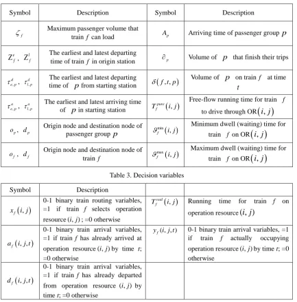
i j,

Table 3. Decision variables

Symbol Description

 

,

f

x i j

0-1 binary train routing variables, =1 if train f selects operation resource( , )i j ; =0 otherwise

 ,

real f

T i j Running time for train f on operation resource( , )i j

, , 

f a i j t

0-1 binary train arrival variables, =1 if train f has already arrived at operation resource( , )i j by time t; =0 otherwise

( , , )

f

y i j t 0-1 binary train arrival variables, =1 if train f actually occupying operation resource( , )i j by time t; =0 otherwise

, , 

f d i j t

0-1 binary train arrival variables, =1 if train f has already departed from operation resource ( , )i j by time t; =0 otherwise

C. Medium-speed Maglev Train Timetabling with Consideration of Passenger Demands

As before mentioned, the objective of minimizing the total travel time of passengers is addressed in this paper. The MSM train timetabling model based on cumulative flow variables is formulated as follows.

min _{p p}

p P f F

Z t

 



 

  ₍₁₎

Where,

:( , ) ( )

( , , ) ( , , 1)

D

p p f

p f p f p p

t i i d E d E

t t a i d t a i d t A



 

 







_   _

Subject to

Group 1: Flow balance constraints

Flow balance constraints at the origin node, intermediate nodes, destination node.

, :( , ) ( )

( , ) 1, O

f f

f

i j i j E o E

x i j f



 



(2)

:( , ) ( ) :( , ) ( )

( , ) ( , ), ,

D O

f f

f f f f

i i j E j E k j k E j E

x i j x j k f j N o d

 

    

, :( , ) ( )

( , ) 1,

D f f

f i j i j E d E

x i j f



 



(4)

Group II: Running time and dwell time constraints

Running time constraints: Real running time cannot small than free-flow running time.

 ,



, ,  , , 1





, ,  , , 1



, , , 

real

f f f f f f

t t

T i j 



t_d i j t d i j t _ 



t_a i j t a i j t _ f i j E (5)

( , ) ( , ), , ( , )

real pure

f f f

T i j T i j f i j E (6) Minimum and maximum dwell time constraints.

           

min _, pure _, real _, max _, pure _{, , , ,}

f i j Tf i j Tf i j f i j Tf i j f i j Ef Wf

       (7)

Group III: Time-space network constraints

Mapping constraints between time-space network and physical network.

( , ) ( , , T), , ( , )

f f f

x i j a i j f i j E (8)

Starting time constraints at origin node.

:( , )

( , , ) 0, ,

f f

e

f f f

j o j E

a o j t f t



   



(9)

:( , )

( , , ) 0, ,

f f

e

f f f

j o j E

d o j t f t



   



(10) Cell-to-cell transition constraints.

, :( , ) , :( , )

( , , ) ( , , ), , ,

f f

f f f f

i j i j E j k j k E

d i j t a j k t f j N o d t

 

    





(11)

Group IV: Passenger demands constraints

Passenger pickup service uniqueness constraints: Each passenger is picked up and dropped off exactly once by a train.

 

  ,

, , , ,

, , 1, , ,

p f

d d

f e p l p

f F i j t

y i j t p t  

 

 

  _{  }

 

(12)

 

  ,

, ,

, ,

, , 1, , ,

p f

a a

f e p l p

f F i j t

y i j t p t  

 

 

  _{  }

 

(13) Passenger to train assignment volume constraints: identify the volume of passengers regarding OD pair p that have finished their trip.



 



,

, ,

:( , ) ( )

= , , , , , , ,

D p p p f

a a

p f e p l p

f F i i d E d

y i j t  f t p p t  

  

 







  _{  } (14)

Capacity constraints: Ensure that passenger volume on train f not exceeding the maximum passenger capacity.

   , ,

, , , ,

p f

f f

i j

y i j t  p f



 



(15)

Group V: Capacity constraints

Cell occupancy indication constraints: Represent the spatial occupancy of train f .











'



, , , ,

, , , , , , ,

f f f i j f f i j

y i j t a i j th d i j th ，f t (16)



_{, ,}



_{1, ,} '_, f

f F

y i j t f f t



 



(17)

Group VI: Time connective constraints for cumulative flow variables

If train f has arrived at or departed from R i j

 

, by timet, thena_fi j t, , or d_fi j t, , has to have a

value of 1 for all later time periods.



, , 1





, , ,



,

f f

a i j t a i j t f t (18)



, , 1





, , ,



,

f f

d i j t d i j t f t (19)

Solution Method

In the process of model establishment, this paper adds the capacity constraint of OR. The same OR involves the interaction between trains, which is difficult to solve, and needs to be relaxed, and add it as a penalty term to the objective function [9]. So this paper uses Lagrange relaxation (LR) algorithm to solve the problem.

A group of non-negative Lagrange multiplier i j t, , are introduced to relaxed OR capacity constraint (17), and add it as a penalty term to the objective function, the changed objective function as following

  , ,  

,

min _{p p}+ _{i j t f} , , 1

p P f F i j t f F

Z D t  y i j t

  

 

   _  _

 

 





(20) Where, i j t, , represents the cost that trains occupying ( , )i j at time t.

Constantly changing the objective function (21):

 

, ,

,

min f i j t f F i j t

Z D L 











(21)

Where,  

 , , ,

+ , ,

f

f p p i j t f

p P i j E t

L t  y i j t

 





 

 

 (22)

Equation (22) consists of two parts, the sum of time benefit and the Lagrange multiplier of the trains occupying the OR (resource price). The solution to the sub-problem that violates the capacity constraint is punished through the Lagrange multiplier. Relaxation constraints enlarge the feasible domain of the solution, and even the infeasible solutions may appear, so the heuristic algorithm are used to transform the infeasible solution into a feasible solution.

The termination condition of the algorithm as follows:

(1) Set maximum number of iterationsI_max, if rImax, the algorithm is terminated;

(2) When iteration number rImax, but the gapεbetween upper and lower bound is small than or

equal to the preset minimum gapε*, the algorithm is terminated.

Original problem model

Relaxation model

The Lagrange multipliers is introduced to relax the complex constraints

Subproblem Lower bound Shortest path algorithm Upper bound Heuristic algorithm

Compute the gap between lower bound

and upper bound

*

ε ε

max

rI

[image:6.595.192.405.68.236.2]

Output optimum solution Update Lagrange multiplier No No Yes Subgradient algorithm Yes

Figure 4. Solving process of LR algorithm.

Example

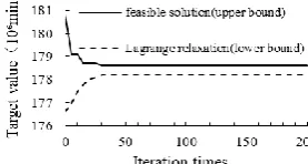
[image:6.595.247.347.392.476.2] [image:6.595.190.407.501.672.2]

The model and algorithm in this paper are verified by a line with 8 stations. The time horizon is 4 hours, from 7:00 am to 11:00 am and the time interval is 1 minute. Cumulative passenger flow distribution is shown in Figure 5. According to the same passenger group with the same OD, expecting departure and arrival time, 5290 passengers are divided into 79 passenger groups. According to trains’ arrival and departure time obtained from the algorithm, train diagram shown in Figure 6. Figure 7 shows the iterative process of the LR algorithm, andr200. The model begins to converge after 36 iterations, and the gap of upper and lower bound is 0.89%.

Figure 5. Cumulative distribution diagram of passenger flow in different time periods.

7 8 9 10 11

Station 1 Station 2 Station 3 Station 4 Station 5 Station 6 Station 7 Station 8 1 3 5 3 5 0 3 7 0 2 4 9 1 0 8 0 1 9 1 6 7 2 3 5 7 2 3 2 1 3 4 2 4 9 1 6 7 9 0 5 7 6 4 6 0 8 2 7 9 4 6 8 0 5 7 6 0 2 3 1 4 9 1 6 7 9 0 5 6 5 4 6 8 6 8 3 5 0 2 4 6 1 2 1 7 9 1 9 1 6 8 3 5 7 9 4 6 8 2 4 5 3 5 0 2 7 9 1 3 8 0 9 0 2 3 1 2 7 8 3 4 6 7 2 3 2 3 5 6 4 5 0 1 6 7 9 0 5 6 5 6 8 0 8 0 5 7 2 4 6 8 3 5 4 4 6 7 5 6 1 2 7 9 1 2 7 8 7 7 9 1 9 2 7 9 4 6 8 0 5 7 6 1 23 4

0 5 8 6 3 7 5

[image:6.595.227.366.699.773.2]

8 910111213

Figure 6. Train timetable obtained by algorithm.

Through the model and algorithm constructed in this paper, the train diagram is roughly corresponding to the distribution of passenger flow. A total of 74 passenger groups have been served within the set time period. As the impact of the expecting time window, there are 63 passengers unfinished travel, accounting for 1.2%.

Conclusion

In this paper, we combine the passenger flow scene of medium-speed maglev traffic and characteristics of line condition, proposed a method of MSM train timetabling with consideration of passenger demands, which is solved by Lagrange relaxation algorithm framework. Finally, the example results show that the model proposed in this paper is feasible to solve the problem of the influence of auxiliary stopping area and power supply area, and this method can effectively solve the passenger's demand for time and space in medium-speed maglev traffic.

Acknowledgment

The authors acknowledge the financial support of the National Key R & D Program of China (2016YFB1200601).

References

[1] Niu H, Zhou X. Optimizing urban rail timetable under time-dependent demand and oversaturated conditions [J]. Transportation Research Part C, 2013, 36(11):212-230.

[2] Robenek T, Maknoon Y, Azadeh S S, et al. Passenger centric train timetabling problem [J]. Transportation Research Part B, 2016, 89:107-126.

[3] Robenek T, Azadeh S S, Maknoon Y, et al. Train timetable design under elastic passenger demand [J]. Transportation Research Part B Methodological, 2018, 111:19-38.

[4] Niu H, Zhou X, Gao R. Train scheduling for minimizing passenger waiting time with time-dependent demand and skip-stop patterns: Nonlinear integer programming models with linear constraints [J]. Transportation Research Part B, 2015, 76:117-135.

[5] Huang Y, Yang L, Tang T, et al. Saving Energy and Improving Service Quality: Bicriteria Train Scheduling in Urban Rail Transit Systems [J]. IEEE Transactions on Intelligent Transportation Systems, 2016, PP(99):1-16.

[6] Zhang W, Wei W, Yang Y, et al. An Operation Control Strategy for the Connected Maglev Trains Based on Vehicle-Borne Battery Condition Monitoring[J]. Wireless Communications & Mobile Computing, 2018, 2018(4):1-10.

[7] Zhang Qi-liang, Chen Yong-sheng. Working diagram algorithm of maglev train [J]. Journal of Computer Application, 2011, 31 (3): 812-814.

[8] Zhang Qi-liang, Chen Yong-sheng, Du Lei. Method for drawing double-track high-speed maglev train diagram based on knitting algorithm [J]. Journal of Computer Application, 2011, 31 (12): 3434-3437.